If you wish to contribute or participate in the discussions about articles you are invited to contact the Editor
Coherent Adaptive Sub-Carrier Modulation (CASM) and Interplex
| Fundamentals | |
|---|---|
| Title | Coherent Adaptive Sub-Carrier Modulation (CASM) and Interplex |
| Author(s) | J.A Ávila Rodríguez, University FAF Munich, Germany. |
| Level | Advanced |
| Year of Publication | 2011 |

Origins of CASM and Interplex
The CASM Modulation is very similar to Interplex [S. Butman and U. Timor, 1972][1]. It receives also the name of Modified Tri-code Hexaphase modulation since it can be seen as a constant envelope modification of the Tri-code Hexaphase modulation. CASM was first proposed in [M. Ananda et al., 1993][2] and later patented by [P.A. Dafesh, 2002][3]while Interplex was patented by [G.L. Cangiani, 2005][4].
In spite of CASM and Interplex being mathematically very similar, an important distinction must be made regarding the implementation. In fact, while Interplex uses exclusively additive methods to multiplex the signals, CASM employs a combination of angle modulation and additive methods. In the end, both of these techniques require the addition of an Inter-Modulation (IM) component that is necessary to maintain constant carrier magnitude [A. R. Pratt and J. I. R. Owen, 2007][5]. It is therefore important to keep in mind that while in the next pages we will refer indistinctly to CASM and Interplex since they are very similar from the mathematical point of view, they are realized and implemented in two very different ways, with two associated patents. In fact, CASM is described in [P.A. Dafesh, 2002][3], while Interplex was presented later by [G.L. Cangiani, 2005][4]. The slight differences between both implementations are also reflected in the performance during the amplification, where CASM is more subject to non-desired effects.
CASM and Interplex are constant envelope modulations with added sub-carriers that do not distort the existing ones when the composite signal is passed through a high-power amplifier operating close to saturation. Moreover, they provide additional control on the power and the spectral separation of the different quadrature multiplexed signals through the use of different sub-carrier frequencies, a particular sub-carrier code rate and a sub-carrier modulation index. As we have emphasized in the previous chapters, this is especially interesting when a high number of signals must be transmitted on the same band. In addition, the modulation of orthogonal pairs of sub-carrier signals on the I and Q phases is also possible with reduced distortion and losses.
The CASM and Interplex implementations provide a means to multiplex all the signals that is equivalent to the spatially combined transmitter implementation of the Linear Modulation. In fact, CASM and Interplex have only slightly higher modulation losses than the Linear Modulation, but can work in saturation achieving thus in the end a superior efficiency for the same total required power. It is also important to keep in mind that although using a separate aperture would in principle provide the cleanest transmission of all the signals, the simplification in the modulator design that using an unique constant envelope allows is more than offset by the impact on the satellite of adding an independent antenna and amplifier.
Finally, it is interesting to note that as stated in the CASM patent [P.A. Dafesh, 2002][3], the Inter-Modulation (IM) signals could be used as additional ranging or communication signals, transmitting thus additional information to that of the data channels. This is indeed the point where some people make another difference between CASM and Interplex. According to this, CASM would use the Inter-Modulation signals as another useful signal to transmit, while the Interplex implementation would allocate such a low power on this component that can be seen as lost power. Finally it is important to underline that the patent of [G.L. Cangiani, 2005][4] incorporates CASM but it is actually directed to a multi-beam/multi-antenna invention.
CASM, Interplex and Modified Tri-Code Hexaphase
CASM and Interplex can be seen as particular cases of the QPSM modulation or as an evolution of the conventional constant-envelope sub-carrier modulation. It is important to stress again that while Interplex uses exclusively additive methods to multiplex the signals, CASM employs a combination of angle modulation and additive methods. Moreover, CASM can utilize the cross-product inter-modulation (IM) terms as an additional useful signal. These terms can be considered as new ranging communication signals in some applications and not only as noise in the most general case. Nevertheless, for our navigation applications these terms will not be desired.
This modulation is extremely flexible and efficient, offering additionally the possibility to provide modes of operation with civilian and military signals together. This makes the approach of great interest. In addition, CASM and Interplex provide high efficiency with values greater than 90% and inherent flexibility to fine tune the modulation architecture maintaining an ability to provide backward compatibility with current signals [G.L. Cangiani, 2005][4]. Also of great interest is that they may be generated using both square-wave and sine-wave sub-carriers although employing square-wave signals is normally preferred.
As shown in [A.R. Pratt and J.I.R. Owen, 2005][6] and [G.L. Cangiani, 2005][4], the CASM and Interplex techniques are able to support altogether more complex solutions than any of the techniques studied so far. In fact, if we work with equation (1) derived for the general Quadrature Product Sub-carrier Modulation (QPSM) case,
and assume that there is a single sub-carrier, the expression can be rewritten as follows:
where m is the modulation index of the multiplex, [math]\displaystyle{ s_c\left(t\right) }[/math] the modulating signal and [math]\displaystyle{ \phi_s\left(t\right) }[/math] the periodic sub-carrier. This expression can be further developed as follows:

yielding:

This can also be expressed in a simplified form as follows:
with

where the in-phase and quadrature components have been isolated. Moreover, if we carefully look at the equation above, we can recognize that the envelope is constant, as it could not be different since the single sub-carrier case is a particular case of the general QPSM modulation where we have shown that this is true.
In navigation the in-phase [math]\displaystyle{ I_0 }[/math] and quadrature [math]\displaystyle{ Q_0 }[/math] signals are modulated with data and pseudorandom codes. The signal modulated with data and code is called data channel while the other one has only code and is thus known as data-less or pilot channel. According to this, we have:

In addition, the sub-carrier modulating signal [math]\displaystyle{ s_c\left(t\right) }[/math] can be considered to contain data [math]\displaystyle{ d_s\left(t\right) }[/math] and spreading code [math]\displaystyle{ c_s\left(t\right) }[/math]. Moreover, this signal is further modulated by the so-called data and code partitioning functions d(t) and c(t) correspondingly [A.R. Pratt and J.I.R. Owen, 2005] [6], depending on whether the term modulates the data or the code. We can write thus:
These two partitioning functions are of great importance since they control the type of QPSM modulation that we will have, as shown in [P.A. Dafesh, 1999a][7] and P.A. Dafesh, 1999b][8]. If we assume, a square-wave sub-carrier we have then:
where we have to note that the square-wave works with a frequency [math]\displaystyle{ f_s }[/math]. In addition, if the signal [math]\displaystyle{ s_c\left(t\right) }[/math] is binary, we can simplify for this particular case as follows:

If we substitute now in (5) we have then:

where

As we have already commented above, depending on the values that the functions [math]\displaystyle{ \alpha_d\left(t\right) }[/math] and [math]\displaystyle{ \beta_c\left(t\right) }[/math] adopt, we will have the different QPSM options identified by [A.R. Pratt and J.I.R. Owen, 2005][6] and [P.A. Dafesh et al., 2006][9]. If we take a closer look at the equations, we can recognize the desired in-phase and quadrature components of s(t) multiplied by cos(m) while the additional non-desired components added by the sub-carrier modulation appear multiplying sin(m). We have assumed from the very beginning that the data and code spreading codes are binary, and thus a useful multiplex option is shown to be the one that results from further assuming the following values for the partitioning functions:

These partitioning functions make use of the binary characteristics of the codes and data to separate them. In fact, substituting in (11), we obtain the following identities:

Moreover, assuming that the codes [math]\displaystyle{ c_I\left(t\right) }[/math] and [math]\displaystyle{ c_Q\left(t\right) }[/math] are optimized to be orthogonal with each other, as it is the case, and that the I and Q data signals are also independent and thus ideally orthogonal, we can rename the terms [math]\displaystyle{ c_{QS}\left(t\right) }[/math] and [math]\displaystyle{ d_{QS}\left(t\right) }[/math]as [math]\displaystyle{ c_{S,IM}\left(t\right) }[/math] and [math]\displaystyle{ d_{S,IM}\left(t\right) }[/math] correspondingly, where the term IM denotes the Inter-Modulation signal. Finally, applying the changes described above, our multiplexed signal s(t) can be expressed as follows:

It is interesting to note from the expression above that the original quadrature product components are reduced by a factor cos(m). We recall that these quadrature product components could correspond to two already existing orthogonal signals as could be the C/A Code and the P(Y) Code in GPS (CASM implementation) before the M-Code was introduced. But also Galileo with Interplex follows a similar pattern with the OS signals in-phase and the PRS in quadrature. In addition, we can see a new sub-carrier component with a BOC modulation and data [math]\displaystyle{ d_s\left(t\right) }[/math] and code [math]\displaystyle{ c_s\left(t\right) }[/math]. Finally, we can equally recognize a fourth component with the codes and data signals [math]\displaystyle{ c_{S,IM}\left(t\right) }[/math] and [math]\displaystyle{ d_{S,IM}\left(t\right) }[/math]. Since this last signal does not transmit any useful information in the general case as it is modulated by the cross-correlation of two codes that are ideally orthogonal and two data streams that in an ideal case are also independent, this term is further called inter-modulation component. Nonetheless, it must be noted that if an appropriate structure were found for the 3 spreading codes [math]\displaystyle{ c_I\left(t\right) }[/math],[math]\displaystyle{ c_Q\left(t\right) }[/math] and [math]\displaystyle{ c_s\left(t\right) }[/math], this could be used as a fourth channel to transmit an additional signal.
In summary, CASM and Interplex offer a QPSK signal and an additional BOC, all of them forming a constant envelope multiplexed signal. The phase constellation diagram is given by the following 8 points:

and the power of the different channels is thus:

We can further analyze the equations if we recall again the equation that we derived above:

where

We can further project the amplitudes of each of the signals on the I and Q axes, such that:

where P is the total power of the signal and [math]\displaystyle{ \beta }[/math] an additional variable to link the I and Q powers, [math]\displaystyle{ P_I }[/math] and [math]\displaystyle{ P_Q }[/math] respectively. Furthermore, we rename the variables [math]\displaystyle{ \beta }[/math] and as follows:

and redefine the signals as follows:

We can show that then:
yielding thus,
which can be further simplified to:

If we introduce these expressions in (17), we have then:

which coincides with the form derived by [E. Rebeyrol et al., 2005]. In fact, it is not difficult to show that after some math this expression can be further simplified to:

where the factor multiplying the signal [math]\displaystyle{ s_1\left(t\right) }[/math], namely [math]\displaystyle{ \beta_1 }[/math], is equal to [math]\displaystyle{ - \pi/2 }[/math] so that this signal is in quadrature with the other two we want to modulate, namely [math]\displaystyle{ s_2\left(t\right) }[/math] and [math]\displaystyle{ s_3\left(t\right) }[/math]. Moreover, the normalized powers of the different signals can be expressed as follows:

According to this, the modulated signal could be generated following the scheme shown in [G.L. Cangiani and J.A. Rajan, 2002] [10]:

The generation scheme presented above is conceptually useful to derive the theoretical expressions of this chapter but presents a series of limitations in a real implementation as identified by [G. L. Cangiani et al., 2002] [11].
While common practice in the design of the architecture dictates generating the entire composite signal at baseband first to further up-convert it later to the desired carrier frequency, for the frequencies of interest in GNSS (microwave systems) this is a problem. In fact, the baseband frequency is too low to avoid harmonic and intermodulation interference with the desired output during the up-conversion. Moreover, the time jitter of the Digital-to-Analog Converters (DAC) adds phase noise onto the desired output signal and the up-conversion process requires band-pass filters at each mixing stage that destroy the original constant envelope of the signal.
A solution to this problem is the implementation proposed by [G. L. Cangiani et al., 2002] [11] where the Interplex signal at the desired carrier frequency is generated as depicted in the following figure.
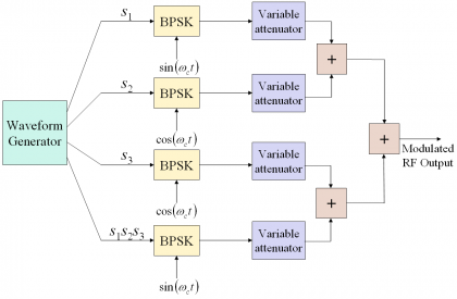 Figure 2: Alternative Interplex scheme proposed by [G. L. Cangiani et al., 2002] [11].

As an example, the variation of the signal power of s1 as a function of the two interplex modulation angles [math]\displaystyle{ \beta_2 }[/math] and [math]\displaystyle{ \beta_3 }[/math] is shown in the following figure:

As we can see, the optimum combination of [math]\displaystyle{ \beta_2 }[/math] and [math]\displaystyle{ \beta_3 }[/math] depends on how much power we want to place on each of the desired signals. In fact, the principle is to minimize the amount of power of the IM channel since this does not bring any information.
It must be noted that the equations derived above do not make use of the data and code partitioning functions. We express now the equivalent form for baseband as follows:

As we can recognize, the equations derived above are based on the assumption of binary data and spreading codes, and a square-wave sub-carrier signal (BOC). Accordingly, the results are not valid for the most general case but can be easily generalized to other types of signal waveforms at the extent of some extra terms in the final expressions. Indeed, as we will show next, adapting this multiplexing to include the CBOC implementation of the MBOC signal is trivial. Furthermore, the derived expressions are only valid for infinite bandwidth, being thus the real power split among all the signals slightly different after filtering.
If we further normalize (28) to have unit power, the previous expression adopts the following form:

which can be further simplified as follows:

For simplicity we refer next all the powers to [math]\displaystyle{ P_3 }[/math]. In fact, to define uniquely the multiplex with three signals, two power ratios are necessary if the powers are referred to a third signal and the total power sums to unity. According to this, the three-signal interplex is defined by:

being the efficiency of the interplex modulation as follows:

This is the percentage of power with respect to the total transmitted power that is employed for the useful signal.
Finally, it is important to mention that additional signals can be incorporated into the CASM and Interplex schemes because the desirable constant envelope characteristic remains unchanged independent from the shape of the sub-carrier modulation. The drawback is the extra complexity that is needed to separate spectrally the additional signals, as pointed out in [A.R. Pratt and J.I.R. Owen, 2005][6] and developed in [T. Fan et al, 2005]. A particular realization with non-binary sub-carriers is discussed in the next section, where a sinewave sub-carrier is employed instead of the usual square-wave version.
Single Sinewave Sub-carrier CASM
The Single Sinewave Sub-carrier version was originally proposed as a constant-envelope Multi-Mode Spread-Spectrum Sub-carrier Modulation (MMSSS) for GPS [P.A. Dafesh et al., 1999a] [7]. This sub-carrier is shown to adopt the following form:
If we introduce now the sine-wave sub-carrier in equations (34) and (35)
the multiplexed signal is shown to approximate to the following [P.A. Dafesh et al., 1999a][7]:

where [math]\displaystyle{ J_n\left(m\right) }[/math] is the Bessel function of order n and m the modulation index of the signal. As we can recognize, the previous expression is only approximate as an infinite number of carrier harmonics [math]\displaystyle{ \left(J_0,J_2,J_4,\cdots \right) }[/math] and sub-carrier harmonics [math]\displaystyle{ \left(J_1,J_3,J_5,\cdots \right) }[/math] would be required to define the multiplexed signal completely. However, only the first carrier and sub-carrier harmonics need to be considered if [math]\displaystyle{ m \le \pi/2 }[/math]. This will be assumed in the following lines. Furthermore, for this range of modulation index the sinewave CASM approach presents a high efficiency of approximately 95% as shown in [P.A. Dafesh et al., 1999a] [7].
We can further develop the previous expression if we realize the same transformation as in (18). In fact, after some math (36) is shown to simplify to [P.A. Dafesh, 1999a][7]:

It is interesting to note that by appropriately selecting the sub-carrier and code partitioning functions we may employ [math]\displaystyle{ C_{IS}\left(t\right) }[/math] and [math]\displaystyle{ C_{IS}\left(t\right) }[/math] as coherently military acquisition and tracking signals as suggested by [P.A. Dafesh et al., 1999a][7]. Moreover, if different partitioning functions are selected, the I/Q phasing of these military signals can be reversed.
Generalization to any number of Sub-carriers
In the previous chapter, general expressions were derived for CASM and Interplex with only three ranging signals. However, they can be easily extended to any number n of signals in the most general case. Furthermore, the sub-carriers do not necessarily have to be square-wave but could also be sinewaves as shown by [P.A. Dafesh et al., 1999a][7]. In fact, if we recall the general expression:
with

we can see that the number of sub-carriers n that can be multiplexed is in principle unlimited. As we can recognize from the previous expression,
- [math]\displaystyle{ m_i\left(t\right) }[/math] indicates the modulation index of the i-th sub-carrier,
- [math]\displaystyle{ d_i\left(t\right) }[/math] is the data sequence of the i-th multiplexed sub-carrier,
- [math]\displaystyle{ \alpha_d^i\left(t\right) }[/math] is the data partition function of the i-th multiplexed sub-carrier,
- [math]\displaystyle{ \beta_c^i\left(t\right) }[/math] is the code partition function of the i-th multiplexed sub-carrier and
- [math]\displaystyle{ \phi_i\left(t\right) }[/math] is the i-th sub-carrier.
After appropriate selection of the data and code partition functions, (39) can be further modified and expressed as follows for the case of square-wave sub-carriers:
with
being
- [math]\displaystyle{ \phi_i\left(t\right) }[/math] the square-wave sub-carrier,
- [math]\displaystyle{ d_i\left(t\right) }[/math] is the data message of the i-th signal to multiplex, and
- [math]\displaystyle{ c_i\left(t\right) }[/math] is the spreading code of the i-th multiplexed signal.
As we can recognize, this is the same notation that we followed in (26) for the particular case of only three signals to multiplex.
Once we have described CASM and Interplex, it is the right moment to talk a little bit more on the Galileo multiplex needs. Indeed, sometimes we are not free to choose how we want our system to be and in the case of Galileo there were clear requirements and constraints on how the signals should interact with each other. As we will see, this determines already to a high degree the multiplex scheme to choose.
To conclude, it is important to mention that the names Interplex and CASM are ambiguously used to define a similar idea. Nonetheless, we can find slight differentiations in addition to the implementation aspects we have mentioned. In [E. Rebeyrol et al., 2006][12], for example, we can see CASM defined as a three components Interplex modulation with a particular and optimal choice of the modulation indexes. However, nothing is said about what signals are in phase or in quadrature. In fact, although [P.A. Dafesh et al., 1999] [7] and [P.A. Dafesh et al., 2000][13] proposed to have the C/A Code and M-Code in phase with the P(Y) Code in quadrature, other works have explored alternative configurations [G.H. Wang et al., 2004] [14]. The same applies to Galileo as we see next.
Galileo Multiplex Needs
As shown in [A.R. Pratt and J.I.R. Owen, 2005][6], Galileo has to use an additive multiplexing technique that produces a constant envelope by means of an inter-modulation signal. We have shown that this is possible with the Interplex or CASM techniques provided that the modulating signals remain binary. Moreover, the Galileo system aims at having the following signals on E1, for example:
- E1 OS data signal,
- E1 OS pilot signal,
- E1 Public Regulated Service (PRS), and
- an Inter-Modulation (IM) signal.
Interplex fulfils these requirements and it is in fact the multiplex baseline for the Galileo signals transmitted on E1 as shown in [G.W. Hein et al., 2002][15] and [G.H. Wang et al., 2004] [14].
The Interplex modulation consists of one In-phase and one quadrature signal. In the particular case of Galileo:
- The In-phase signal is the linear sum of the two Open Signal components, OSD and OSP where D stands for data and P for pilot.
- The quadrature signal carries the Public Regulated Service (PRS) signal and an additional signal, named inter-modulation product, whose role is to provide the modulation with a constant envelope.
Moreover, according to [Galileo SIS ICD, 2008][16], the power split of the OSD, OSP and PRS must be 25 %, 25 % and 50 % respectively.
As we have seen in chapter CBCS Modulation, the mathematical expression of the interplex modulation for the old BOC(1,1) baseline of 2004, it is shown to be:


where,
- [math]\displaystyle{ A_0 }[/math] is the amplitude of the modulation envelope,
- [math]\displaystyle{ \theta\gt _0 }[/math] is the angle of four of the six phase states of the 6-PSK modulation. It corresponds to half the angular distance between 2 states across the real axis,
- [math]\displaystyle{ S_{BOC_{\left(1,1\right)}}\left(t\right) }[/math] represents the BOC(1,1) modulation,
- [math]\displaystyle{ S_{PRS}\left(t\right) }[/math] is the PRS BOCcos(15,2.5) modulation,
- [math]\displaystyle{ S_{IM}\left(t\right) }[/math] is the Inter-Modulation product, used to keep the amplitude constant, and
- [math]\displaystyle{ c_D\left(t\right) }[/math] and [math]\displaystyle{ c_p\left(t\right) }[/math] are the codes for the E1 OS data and pilot channels respectively.
The baseband equations above can also be expressed as follows for the particular case of the Galileo signals on E1:

being

Here the coefficients [math]\displaystyle{ \alpha,\beta }[/math] and [math]\displaystyle{ \gamma }[/math] play the same role as the phase angles [math]\displaystyle{ \theta_0 }[/math] and the amplitude [math]\displaystyle{ A_0 }[/math] in the equations of previous chapters. Moreover, D stands for data, P for pilot, [math]\displaystyle{ d\left(t\right) }[/math] is the data signal, [math]\displaystyle{ c\left(t\right) }[/math] is the PRN code and [math]\displaystyle{ s\left(t\right) }[/math] is the modulated signal. As it can be shown, the resulting modulation is a 6-PSK or Hexaphase modulation with constant envelope, also known as Modified Hexaphase for this reason. Next figure shows the phase plot:

where the angle [math]\displaystyle{ \theta_0 }[/math] is chosen so as to provide the appropriate power ratio as described in the Power Spectral Density of the CBCS Modulation. In our case, in order to have the power ratios given in [Galileo SIS ICD, 2008][16], the value must be of:
To have a better understanding on the location of the phase states, we show next the different probabilities of the constellation phase points by means of the following truth table. It must be noted that the amplitudes were not corrected to account for the loss of efficiency that results from the inter-modulation signal IM.

We can graphically see this also as follows:

As we can see from the figure and table above, states 2 and 5 occur each with a probability of 25%. As a result, the OS channel transmits no signal 50 % of the time. Moreover, binary codes were assumed with values {+1,-1} of equal probability. In addition, the PRS has 3 dB more power than the OS signals in consonance with [Galileo SIS ICD, 2008][16]. As we can see, the mission of the Inter-Modulation signal IM is to bring the phase points back to the circle as depicted by the arrows of the figure above.
The final power distribution inside the modulation takes thus the following values for the baseline of 2004:

As we can observe, the IM term has a power level of -9.54 dB with respect to the total transmitted power and 6 dB below the PRS. It is important to note that in a real application the values derived above should be further compensated to account for the different losses of every signal through the satellite filter.
Moreover, the amplitude of the envelope, [math]\displaystyle{ A_0 }[/math], must be modified to compensate the loss of efficiency of the modulation due to the presence of the Inter-Modulation product. In the present case, [math]\displaystyle{ A_0 }[/math] is set to [math]\displaystyle{ \sqrt{9/8}=1.0607 }[/math]. After applying the amplitude compensation, the power distribution adopts the following form:

Finally, it is interesting to note that the power split between the OS and PRS channels can be easily modified playing with the parameters [math]\displaystyle{ A_0 }[/math] and [math]\displaystyle{ \theta_0 }[/math]. In terms of phase states, the effect would be a movement of the phase angle [math]\displaystyle{ \theta_0 }[/math] within the circle of the constellation.
Power Spectral Density of CASM and Interplex
Although CASM and Interplex correspond to two different implementations, the simplified mathematical description is very similar, being only the Inter-Modulation components slightly different. As we have seen in the lines above, the baseband expression can be expressed as:

where

Moreover, as shown in [E. Rebeyrol et al., 2006][12]
such that:

As shown in Power Spectral Density of the AltBOC Modulation, the autocorrelation of the baseband signal adopts the form:

If we further assume ideal codes, the expression for the autocorrelation function will be:

In addition, since the power spectral density is the Fourier Transform of the autocorrelation function, we have:
Equally, for the whole signal including carrier frequency, we would have:

CASM Modulation in GPS
If we apply CASM to all the GPS signals except for GPS L1C, the Power Spectral Density is shown to adopt the following form:
where the power spectral densities of the C/A Code, P(Y) Code and M-Code. In the case of the IM component, the signal presents the spectrum of a BOC(10,10) modulation. In fact, as we have already seen, the Inter-Modulation signal is formed by multiplying the three signals we want to modulate. In this case, [math]\displaystyle{ s_1\left(t\right) }[/math] is BPSK(1), [math]\displaystyle{ s_2\left(t\right) }[/math] is BPSK(10) and [math]\displaystyle{ s_3\left(t\right) }[/math] is BOC(10,5). Since the three signals are binary, the product of them will be a sine or cosine-phased [math]\displaystyle{ BOC\left(f_s,f_c\right) }[/math] modulation with [math]\displaystyle{ f_s }[/math] the highest offset carrier frequency of the three and with code rate fc the highest of the three. In this particular case the chipping rate of the P(Y) code and the offset carrier frequency of the M-Code.
Moreover, as presented in [P.A. Dafesh et al., 2000] [13], the GPS CASM modulation defines its angle [math]\displaystyle{ \beta_2 }[/math] as follows:

being thus the only variable to play with the angle [math]\displaystyle{ \beta_3 }[/math] which is renamed as m in this particular case. Consequently, the power of each particular signal depends only on m:

so that
As a conclusion, the CASM GPS signal can thus be expressed as follows:

As we can see, the desired powers and relationships between the different signals, can be well adjusted by appropriately selecting the values of [math]\displaystyle{ \beta_2 }[/math] and m. The corresponding diagram of the modulation constellation is shown in the following figure from [E. Rebeyrol et al., 2006][12].

As we can recognize from equation (59), the phase rotation of the sub-carrier signal onto the carrier can be implemented in very different ways. Apart from implementations of proprietary nature, two main realizations of the CASM modulation have been identified for GPS as identified in [P.A. Dafesh et al., 2000] [13]:
- The most straightforward approach is to process the sub-carrier signal in baseband. According to this, the new signal to add in the multiplexing produces a digital rotation of the phase of the carrier as shown in Figure 7 below:
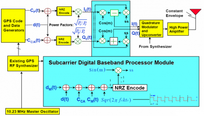 Figure 7: Flexible digital CASM modulator implementation [P.A. Dafesh et al., 2000] [13].

- An alternative implementation is to phase modulate the local oscillator as described in [P.A. Dafesh, 1999b] [8]. This approach is very similar to that followed on the Space Ground Link Subsystem (SGLS. In this case we would only need an additional bi-phase modulator to modulate the cross-term. It must be noted that depending on the sub-carrier frequency of the new signal to multiplex one approach or the other will be more appropriate.
In the previous lines a CASM implementation was applied to multiplex all the GPS baseline signals except for the new GPS L1C. However, the original CASM modulation method for GPS pursued the transmission of not only one military signal, but actually two. In fact, the CASM technique proposed by [P.A. Dafesh et al., 1999a] [7] was applicable to the transmission of Military Acquisition (MA) and Military Tracking (MT) signals in a flexible and efficient manner. The high efficiency approach presented there for combined aperture, that is C/A, P(Y), MA and MT sent through the same upconverter amplifier chain and antenna, was shown to be equivalent to that of the separate aperture, where MA and MT would be transmitted with a separate upconverter, amplifier and antenna from that of C/A and P(Y).
One final point to discuss is the power efficiency of the resulting multiplex. As an example, we show the case of the C/A Code, P(Y) Code and M-Code signals and assume that the Inter-Modulation signal is 2 dB lower power than the M-Code and the P(Y) Code as also done in [P.A. Dafesh et al., 2000] [13]. Furthermore, regarding the filtering losses showed in Table 5,

the power efficiency of CASM in GPS will be:

As we can see, the total transmitted power is approximately the same as that of the Linear Modulation (-151.6 dBW). However, here the result of applying CASM to GPS results in a final efficiency of approximately 79.45 %, or 0.99 dB loss in total power due to the CASM Multiplexing and filtering of the IM signal when only the useful signals are considered. That results in 0.69 dB higher losses than in the case of the Linear Modulation, which had 0.30 dB losses or 93.23 % power efficiency. The efficiency of the CASM approach can be further improved if the Inter-Modulation signal is tracked reaching then a final efficiency of approximately 92%, or 0.36 dB losses. This means only 0.06 dB higher losses than in the case of the Linear Modulation.
We can conclude that the CASM implementation of GPS presents slightly higher modulation losses than the Linear Modulation in general. However, the overall power efficiency when all the contributions are taken into account is significantly greater for CASM than for the Linear Modulation since in this case it is not required that the amplifier works at back-off or that a separate high power amplifier chain is used.
It is important to note that the conclusion from the example above results from a very simplified approach as it is not possible to complete all the modulation at baseband and have just one up-conversion to the transmission frequency. As a result of distributed signal filtering, in reality there are differences in the signal trajectory between the phase plane plots, what has a significant effect on the requirement for HPA back-off. Ideally, a desirable feature would be that all transients lie along the unit circle. However, this does not happen in real implementations in any case.
Interplex Modulation for Galileo: BOC(1,1) + [math]\displaystyle{ BOC_{cos}\left(15,2.5\right) }[/math]
If we apply the Interplex Modulation to the Galileo signals baseline of 2004, the general expression of the Power Spectral Density is shown to adopt the following expression:

where the power spectral densities of the OS and PRS signals were derived in chapter 4.3.2. Moreover, the IM signal will have the same spectrum as the PRS [math]\displaystyle{ BOC_{cos}\left(15,2.5\right) }[/math] as shown by [E. Rebeyrol et al., 2006][12]. It must be noted that these expressions are only valid for the case of having BOC(1,1) as open signal, since as we have repeatedly mentioned in this chapter, the standard Interplex equations are not valid when we consider the CBOC implementation of MBOC, as this is not binary.
As stated in [Galileo SIS ICD, 2008][16], the total power of the Galileo E1 signals should be equally divided between the in-phase and quadrature components. Furthermore, the power of the data and pilot channels should be equal. Using (27), this leads to the following relationship:

For the Galileo Interplex modulation with BOC(1,1) and [math]\displaystyle{ BOC_{cos}\left(15,2.5\right) }[/math], that is the old baseline of 2004, the modulation index m adopts the value [math]\displaystyle{ m=0.1959\pi }[/math] and the expression of the transmitted signal is shown to be [E. Rebeyrol et al., 2006][12]:

where
- is the total power of the signal,
- [math]\displaystyle{ S_{BOC_{cos}\left(15,2.5\right)}\left(t\right) }[/math] represents the cosine-phased BOCcos(15,2.5) signal waveform of the Public Regulated Service (PRS),
- [math]\displaystyle{ S_{BOC\left(1,1\right)}\left(t\right) }[/math] is the BOC(1,1) modulation that was used for the data and pilot Open Service in the baseline of 2004, and
- [math]\displaystyle{ S_{BOC_{cos}\left(15,2.5\right)}\left(t\right)S_{BOC\left(1,1\right)}\left(t\right) S_{BOC\left(1,1\right)}\left(t\right) }[/math] is the Inter-Modulation term that keeps the constant envelope of the multiplexed signal.
According to this:

Equation (62) can be further simplified if we employ the general notation of equations (38) and (40) as shown next:
The resulting diagram of the modulation constellation is shown in the next figure:
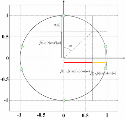 Figure 8: Galileo Interplex phase constellation for the Galileo baseline of 2004 [E. Rebeyrol et al., 2006][12].

Modified Interplex and Modified CASM
As a result of the changes proposed in [G.W. Hein et al., 2005] [17], slight modifications had to be made to the multiplex schemes presented above in order to be able to transmit the CBOC signal for the Galileo E1 OS service. As it can be seen in detail in CBCS Modulation, the CBOC modulation was selected due to its great multipath mitigation potential and spectral compatibility with the rest of signals in the band, among other characteristics of interest. The data and pilot channels are in anti-phase and the difference or additive components are not binary. Indeed, CBOC in particular and CBCS in general, are formed by adding BOC(1,1) with a new sub-carrier, [math]\displaystyle{ S_{BOC\left(6,1\right)}\left(t\right) for CBOC and \lt math\gt S_{BCS}\left(t\right) in general, of relative amplitude \lt math\gt \mu }[/math]. This means that the Inter-Modulation component does not obey to the equations that we saw in the previous lines for Interplex and CASM. However, the Interplex and CASM analytical expressions can be easily modified to account for the new signal waveform. In fact, the composite multiplexed signal should present for CBOC the following form:

being

As we can clearly recognize from the equations above, this modulation scheme is generally more efficient. Indeed, the OS channel is in this case transmitting signal all the time and not only 50 % of the time as was the case with the BOC(1,1) signal. The equation above can be further expressed as follows:

where the emission of BOC(1,1) and the BOC(6,1) signal are shown separately. As it is trivial to recognize, the two emissions are time disjoint and satisfy the requirement to be orthogonal. Another important observation is that now we have 8 phase points instead of only 6. From a quick inspection of the phase diagram one might find analogies with the CASM and Interplex schemes that we saw above. Nonetheless, the CASM and Interplex cannot be applied directly since we do not have binary signals any more.
Finally, it is important to mention that the more signals are multiplexed in the general scheme, the more phase constellation points are needed to achieve the constant envelope. This raises some concerns on the complexity of the signal generator and the identification of the phase points as shown in [A.R. Pratt and J.I.R. Owen, 2005][6]. Indeed, after filtering at the receiver some phase states might be difficult to distinguish if they are too close to each other.
For more details on the modified interplex modulation, refer to [Power Spectral Density of the CBCS Modulation]] where all the analytical expressions for the general CBCS modulation and CBOC are derived.
Interesting Aspects of the Modified Interplex
In all the modulations studied so far, the most typical case was to multiplex binary signals. Nevertheless, there are cases of interest that cannot be described by the original version of the Interplex modulation unless slight modifications are made. In fact, CBOC has data and pilot in anti-phase. This results in an additive/subtractive combination of BOC(1,1) and BOC(6,1) that is not binary any more. Nonetheless, a careful look into the equations shows that for these cases, the inter-modulation still remains binary and thus, except for the amplitude, it can be predicted with the Interplex equations as shown in [G.W. Hein et al., 2005] [17].
Composite BOC (CBOC) requires to form the sum and difference of the data and pilot channels. The conditions for the BOC(1,1) and BOC(6,1) can be stated as follows:

where the BOC(1,1) and BOC(6,1) channels are time disjoint and could be thus separately decoded. The equation above is subject to further interesting interpretations. In fact, since two time multiplexed channels are created, one could use the difference channel to carry additional signals or services as proposed in [A.R. Pratt and J.I.R. Owen, 2005][6]. If we assume that 20 % of the total signal power is on the BCS channel and 80 % on the BOC(1,1) channel, this makes a difference of 6 dB in power. For the bit error rate not to be affected with these power levels, the reduced power of the difference channel BOC(6,1) could be compensated by a reduction of the data rate from 250 symbols per second to 50 as shown next:

being

which is very similar to the expressions derived in previous chapters, but with the slight difference that in this case an additional signal with information [math]\displaystyle{ d_{Diff}^{E1}\left(t\right) }[/math] accompanies BOC(6,1). This additional signal has no effect on the time-multiplexing as we can see, since the phase inversion of this data does only cause a change of the sign of the BOC(6,1) signal at every data symbol transition of the difference channel. Finally, it must be noted that as commented in [A.R. Pratt and J.I.R. Owen, 2005][6], the presence of a data signal on the difference channel, namely BOC(6,1), definitely has an effect on the global signal characteristics equalizing the average spectra, the multipath sensitivity envelope and the DLL tracking characteristics. A method for modulating data for the BOC(6,1) signal and to dispread this data message have been proposed in [A.R. Pratt and J.I.R. Owen, 2005][6].
References
- ^ [S. Butman and U. Timor, 1972] S. Butman and U. Timor , Interplex – An efficient Multichannel PSK/PM Telemetry System, Proceedings of IEEE Transaction on Communications, Volume 20, No. 3 – June 1972.
- ^ [M. Ananda et al., 1993] M. Ananda, M. Munjal, B. Siegel, R. Sung, K.T. Woo, Proposed GPS Integrity and Navigation Payload on DSCS, Proceedings of the IEEE Military Communications Conference, October 1993, Boston, Massachusets, USA.
- ^ a b c [P.A. Dafesh, 2002] P.A Dafesh, Coherent Adaptive Sub-carrier Modulation Method, Patent US 6,430,213, Granted 6 August 2002.
- ^ a b c d e [G.L. Cangiani, 2005] G.L. Cangiani, Methods and Apparatus for Multi-beam Multi-signal Transmission for Actively Phased Array Antenna, Patent US 6856284, granted 15 February, 2005.
- ^ [A. R. Pratt and J. I. R. Owen, 2007] A. R. Pratt and J. I. R. Owen., Signals, System, Method and Apparatus, Patent number WO/2007/148081, International Application No.: PCT/GB2007/002293, Publication date: 27 December 2007
- ^ a b c d e f g h i [A.R. Pratt and J.I.R. Owen, 2005] A.R. Pratt and J.I.R. Owen, Signal Multiplex Techniques in Satellite Channel Availability - Possible Applications to Galileo, Proceedings of the International Technical Meeting of the Institute of Navigation, ION-GNSS 2005, 13-16 September 2005, Long Beach, California, USA.
- ^ a b c d e f g h i [P.A. Dafesh et al., 1999a] P.A. Dafesh, S. Lazar, and T. Nguyen, Coherent Adaptive Sub-carrier Modulation (CASM) for GPS Modernization, Proceedings of the National Technical Meeting of the Institute of Navigation, ION-NTM 1999, January 1999, San Diego, California, USA.
- ^ a b [P.A. Dafesh, 1999b] P.A. Dafesh, Quadrature Product Sub-carrier Modulation (QPSM), IEEE Aerospace Conference Record, March 1999.
- ^ [P.A. Dafesh et al., 2006] P.A. Dafesh, Nguyen, M. Tien, Quadrature product sub-carrier modulation system, Patent US 7120198, Granted 10 October 2006.
- ^ [G.L. Cangiani and J.A. Rajan, 2002] G.L. Cangiani and J.A. Rajan, Programmable Waveform Generator for a Global Positioning System, Patent : US 6335951 granted 1st January 2002.
- ^ a b c [G. L. Cangiani et al., 2002] G. L. Cangiani, R.S. Orr and C.Q. Nguyen, Methods and Apparatus for Generating a Constant-Envelope Composite Transmission Signal, Patent number WO/2002/28044, International Application No.: PCT/US2001/30135, Publication date: 4 April 2002
- ^ a b c d e f [E. Rebeyrol et al., 2006] E. Rebeyrol, C. Macabiau, L. Ries, J.-L. Issler, M. Bousquet, M.-L. Boucheret, Interplex Modulation for Navigation Systems at the L1 band, Proceedings of the National Technical Meeting of the Institute of Navigation, ION-NTM 2006, January 2006, San Diego, California, USA.
- ^ a b c d e [P.A. Dafesh et al., 2000] P.A. Dafesh, L. Cooper, M. Partridge, Compatibility of the Interplex Modulation Method with C/A and P(Y) code Signals, Proceedings of the International Technical Meeting of the Institute of Navigation, ION-GNSS 2000, September 2000, Salt Lake City, Utah, USA.
- ^ a b [G.H. Wang et al., 2004] G.H. Wang, V.S. Lin, T. Fan, K.P. Maine, P.A. Dafesh , Study of Signal Combining Methodologies for GPS III’s Flexible Navigation Payload, Proceedings of the International Technical Meeting of the Institute of Navigation, ION-GNSS 2004, 21-24 September, 2004, Long Beach, California, USA.
- ^ [G.W. Hein et al., 2002] G.W. Hein, J. Godet, J.-L. Issler, J.-C. Martin, P. Erhard, R. Lucas-Rodriguez and A. R. Pratt, Status of Galileo Frequency and Signal Design, Proceedings of the International Technical Meeting of the Institute of Navigation, ION-GNSS 2002, September 2002, Portland, Oregon, USA.
- ^ a b c d [Galileo SIS ICD, 2008] Galileo Open Service Signal In Space Interface Control Document (OS SIS ICD) Draft 1 01/02/2008, 2008, European Space Agency / Galileo Joint Undertaking
- ^ a b [G.W. Hein et al., 2005] G.W. Hein, J.-A. Avila-Rodriguez, L. Ries, L. Lestarquit, J.-L. Issler, J. Godet, A.R. Pratt, Members of the Galileo Signal Task Force of the European Commission: A Candidate for the Galileo L1 OS Optimized Signal, Proceedings of the International Technical Meeting of the Institute of Navigation, ION-GNSS 2005, 13-16 September, 2005, Long Beach, California, USA.
Credits
The information presented in this NAVIPEDIA’s article is an extract of the PhD work performed by Dr. Jose Ángel Ávila Rodríguez in the FAF University of Munich as part of his Doctoral Thesis “On Generalized Signal Waveforms for Satellite Navigation” presented in June 2008, Munich (Germany)