If you wish to contribute or participate in the discussions about articles you are invited to contact the Editor
Kalman Filter
| Fundamentals | |
|---|---|
| Title | Kalman Filter |
| Author(s) | J. Sanz Subirana, J.M. Juan Zornoza and M. Hernández-Pajares, Technical University of Catalonia, Spain. |
| Level | Advanced |
| Year of Publication | 2011 |
The principle of Kalman filtering can be roughly summarised as the weighted least square solution of the linearised observation system augmented with a prediction of the estimate as additional equations. The predicted estimate and the weighted solution are given as follows:
- Predicted estimate (from a simple linear model):
- Let [math]\displaystyle{ \widehat{X}{(n-1)} }[/math] be the estimate for the [math]\displaystyle{ (n-1) }[/math]-th epoch, thence, a prediction for the next epoch [math]\displaystyle{ \widehat{X}^{-}{(n)} }[/math], is computed according to the model [footnotes 1]:
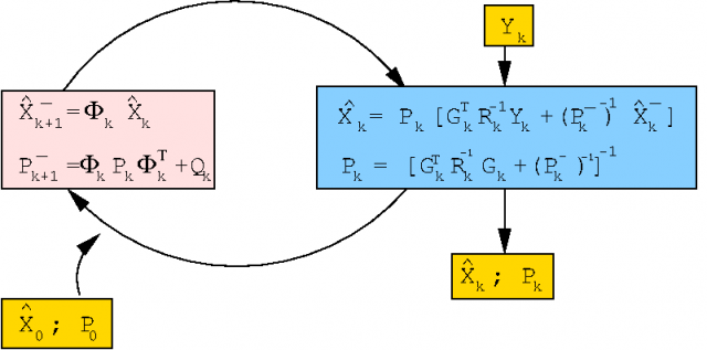
- [math]\displaystyle{ \begin{array}{l} \widehat{\mathbf X}^{-}{(n)}={\boldsymbol \Phi} (n-1)\ \widehat{\mathbf X}{(n-1)}\\[0.3cm] {\mathbf P}_{\widehat{\mathbf X}{(n)}}^{-}={\boldsymbol \Phi} (n-1)\ {\mathbf P}_{\widehat{\mathbf X}{(n-1)}}\ {\boldsymbol \Phi}^T (n-1)+{\mathbf Q}(n-1) \end{array} \qquad \mbox{(1)} }[/math]
- Where [math]\displaystyle{ {\boldsymbol \Phi} }[/math] is named the Transition Matrix and defines the propagation of the vector parameters estimate [math]\displaystyle{ \widehat{\mathbf X} }[/math], and [math]\displaystyle{ {\mathbf Q} }[/math] is the Process Noise Matrix. Matrix [math]\displaystyle{ {\mathbf Q} }[/math] allows, in particular, to add some additional noise to account for possible miss-modelling due to the simple prediction model used or, what is the same, to an inexact description of the problem in general.
- Weighted solution (from measurements and predicted estimate):
- According to the approach of Block-Wise Weighted Least Square the measurements (i.e., the linearised observation equations) are combined with the predicted parameters estimate as follows:
- [math]\displaystyle{ \left[ \begin{array}{c} {\mathbf Y}(n) \\[0.2cm] \widehat{\mathbf X}^{-}(n) \end{array} \right] =\left[ \begin{array}{c} {{\mathbf G}(n)}\\[0.2cm] {\mathbf I} \end{array} \right] {\mathbf X}(n)\ \ ;\qquad {\mathbf P}=\left[ \begin{array}{cc} {\mathbf R}(n) & {\mathbf 0} \\[0.2cm] {\mathbf 0} & {\mathbf P}_{\widehat{X}(n)}^{-} \end{array} \right] \qquad \mbox{(2)} }[/math]
- which is solved as (see Block-Wise Weighted Least Square)
- [math]\displaystyle{ \left[ \begin{array}{c} {\mathbf Y_1} \\ {\mathbf Y_2} \end{array} \right] = \left[ \begin{array}{c} {\mathbf G_1}\\[0.2cm] {\mathbf G_2} \end{array} \right] {\mathbf X} ;\qquad {\mathbf R}=\left[ \begin{array}{cc} {\mathbf R_1} & {\mathbf 0} \\[0.2cm] {\mathbf 0} & {\mathbf R_2} \end{array} \right] \qquad \mbox{(3)} }[/math]
- being the weighted least squares estimate:
- [math]\displaystyle{ \begin{array}{l} {\mathbf P}_{\widehat{X}(n)}=\left[ {\mathbf G}^T(n)\;{\mathbf R}^{-1}(n)\;{\mathbf G}(n)+\left( P_{\widehat{\mathbf X}(n)}^{-}\right) ^{-1}\right] ^{-1}\\[0.3cm] \widehat{\mathbf X}(n)={\mathbf P}_{\widehat{X}(n)} \cdot \left[{\mathbf G}^T(n) \; {\mathbf R}^{-1}(n)\; {\mathbf Y}(n)+\left( {\mathbf P}_{\widehat{\mathbf X}(n)}^{-}\right) ^{-1}\widehat{\mathbf X}^{-}(n)\right]\\ \end{array} \qquad \mbox{(4)} }[/math]
- The algorithm can be summarised in the following scheme [footnotes 2]:
- Using the following relations [1],
- [math]\displaystyle{ \begin{array}{l} (ACB+D)^{-1}=D^{-1}-D^{-1}AMBD^{-1}\\[0.3cm] M=(BD^{-1}A + C^{-1})^{-1} \end{array} \qquad \mbox{(5)} }[/math]
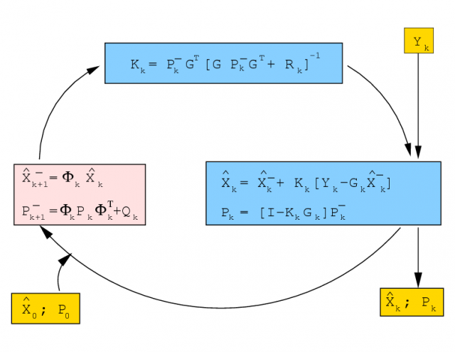
- it can be shown that the previous formulation is algebraically equivalent to the classical formulation of the Kalman filter given by the following figure 2:
Some elemental examples of matrix definitions [math]\displaystyle{ \Phi }[/math] and [math]\displaystyle{ {\mathbf Q} }[/math]
The determination of the state transition matrix [math]\displaystyle{ {\boldsymbol \Phi} }[/math] and Process Noise matrix [math]\displaystyle{ {\mathbf Q} }[/math] is usually based on physical models describing the estimation problem. For instance, for satellite tracking or orbit determination, they are derived from the orbital motion equations. Elemental formulations, i.e., for the SPS and PPP navigation, are covered by the examples given as follows:
Static positioning
The state vector to determine is given by [math]\displaystyle{ \widehat{\mathbf X}=(dx,dy,dz,\delta t) }[/math] where the coordinates [footnotes 3] are considered as constants (because the receiver is kept fixed) and the clock offset can be modelled as a white noise with zero mean. Under these conditions matrix [math]\displaystyle{ \Phi }[/math] and [math]\displaystyle{ {\mathbf Q} }[/math] are given by:
- [math]\displaystyle{ {\mathbf \Phi} (n)=\left[ \begin{array}{cccc} 1 & & & \\ & 1 & & \\ & & 1 & \\ & & & 0 \\ \end{array} \right] \qquad {\mathbf Q}(n)=\left[ \begin{array}{cccc} 0 & & & \\ & 0 & & \\ & & 0 & \\ & & & \sigma _{\delta t}^2 \\ \end{array} \right] \qquad \mbox{(6)} }[/math]
being [math]\displaystyle{ \sigma _{dt} }[/math] the uncertainty in the clock prediction model (for instance [math]\displaystyle{ \sigma _{dt}=1\,ms=300\,km }[/math] for a unknown clock --i.e. [math]\displaystyle{ 1 }[/math] light-millisecond). Notice that the prediction model for the coordinates is exact and, thence, the associated elements in matrix [math]\displaystyle{ {\mathbf Q} }[/math] are null.
Kinematic positioning
- If it is a vehicle running at a high velocity, the coordinates can be modelled as a white noise with zero mean, the same as the clock offset:
- [math]\displaystyle{ {\mathbf \Phi} (n)=\left[ \begin{array}{cccc} 0 & & & \\ & 0 & & \\ & & 0 & \\ & & & 0 \\ \end{array} \right] \qquad {\mathbf Q}(n)=\left[ \begin{array}{cccc} \sigma_{dx}^2 & & & \\ & \sigma_{dy}^2& & \\ & & \sigma_{dz}^2 & \\ & & & \sigma _{\delta t}^2 \\ \end{array} \right] \qquad \mbox{(7)} }[/math]
- If it is a vehicle running at a low velocity, the coordinates can be modelled as a {\it random walk} process with its uncertainty growing with time:
- [math]\displaystyle{ {\mathbf \Phi} (n)=\left[ \begin{array}{cccc} 1 & & & \\ & 1 & & \\ & & 1 & \\ & & & 0 \\ \end{array} \right] \qquad {\mathbf Q}(n)=\left[ \begin{array}{cccc} Q^{\prime}_{dx} \Delta t & & & \\ & Q^{\prime}_{dy} \Delta t & & \\ & & Q^{\prime}_{dz} \Delta t & \\ & & & \sigma _{\delta t}^2 \\ \end{array} \right] \qquad \mbox{(8)} }[/math]
Notes
- ^ It is a first order model of Gauss-Markov. The dynamical character is established through the state transition matrix [math]\displaystyle{ {\boldsymbol \Phi} }[/math] and the noise matrix of the process [math]\displaystyle{ {\mathbf Q} }[/math].
- ^ If one desires to go deeply into the theme, the book [Bierman, 1976] is recommended. Special chapters relating to U-D covariance filter and SRIF.
- ^ We are referring to deviations from nominal values [math]\displaystyle{ (x_0,y_0,z_0) }[/math], that is what it is estimated from the navigation equations.
References
- ^ [Bierman, 1976] Bierman, G., 1976. Factorization Methods for Discrete Sequential estimation. Academic Press, New York, New York, USA.


