If you wish to contribute or participate in the discussions about articles you are invited to contact the Editor
Linear observation model for PPP: Difference between revisions
Carlos.Lopez (talk | contribs) No edit summary |
||
(10 intermediate revisions by 2 users not shown) | |||
Line 1: | Line 1: | ||
{{Article Infobox2 | {{Article Infobox2 | ||
|Category=Fundamentals | |Category=Fundamentals | ||
|Authors=J. Sanz Subirana, J.M. Juan Zornoza and M. Hernández-Pajares, Technical University of Catalonia, Spain. | |||
|Level=Advanced | |||
|YearOfPublication=2011 | |||
|Title={{PAGENAME}} | |Title={{PAGENAME}} | ||
}} | }} | ||
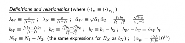
According to the equations described in the [[Combining pairs of signals and clock definition|combination of pairs of signals]] | |||
::[[File: Comb_Pairs_Sign_Fig_1.png|none|640px]] | |||
::[[File: Comb_Pairs_Sign_Fig_2.png|none|640px]] | ::[[File: Comb_Pairs_Sign_Fig_2.png|none|640px]] | ||
Line 31: | Line 30: | ||
where <math>R^j_{_C}</math> is the unsmoothed code pseudorange measurement for the <math>j-th</math> satellite in view and <math>\Phi^j_{_C}</math> is the corresponding carrier measurement. | where <math>R^j_{_C}</math> is the unsmoothed code pseudorange measurement for the <math>j-th</math> satellite in view and <math>\Phi^j_{_C}</math> is the corresponding carrier measurement. | ||
Following the same procedure as in [[Code Based Positioning ( | Following the same procedure as in [[Code Based Positioning (SPS)]], the linear observation model <math>{\mathbf Y}={\mathbf G}\;{\mathbf X}</math> for the code and carrier measurements can be written as: | ||
* '''Prefit-residuals:''' | * '''Prefit-residuals:''' | ||
:<math> | :<math> | ||
Line 50: | Line 51: | ||
''Note:'' The satellite clock offset <math>\delta t^j</math> includes the [[Relativistic Clock Correction|satellite clock relativistic correction]] due to the orbit eccentricity. The [[ | ''Note:'' The satellite clock offset <math>\delta t^j</math> includes the [[Relativistic Clock Correction|satellite clock relativistic correction]] due to the orbit eccentricity. The [[Relativistic Path Range Effect|relativistic path range correction]] is included in the geometric range <math>\rho_0^j</math>.The term <math>T_0</math> is the nominal value for the [[Tropospheric Delay|tropospheric correction]]. | ||
Notice that, and according to the equation | Notice that, and according to the equation | ||
Line 74: | Line 75: | ||
* '''Design matrix''' | * '''Design matrix''' | ||
:<math> | :<math> | ||
{\mathbf G}=\left[ | {\mathbf G}=\left[ | ||
\begin{array}{ccccccccccc} | \begin{array}{ccccccccccc} | ||
\frac{x_0-x^1}{\rho_0^1} & \frac{y_0-y^1}{\rho_0^1} & \frac{z_0-z^1}{\rho_0^1} &1&M_{wet}&0&...&0&...&0\\ | \frac{x_0-x^1}{\rho_0^1} & \frac{y_0-y^1}{\rho_0^1} & \frac{z_0-z^1}{\rho_0^1} &1&M_{wet}^1&0&...&0&...&0\\ | ||
\frac{x_0-x^1}{\rho_0^1} & \frac{y_0-y^1}{\rho_0^1} & \frac{z_0-z^1}{\rho_0^1} &1&M_{wet}&1&...&0&...&0\\ | \frac{x_0-x^1}{\rho_0^1} & \frac{y_0-y^1}{\rho_0^1} & \frac{z_0-z^1}{\rho_0^1} &1&M_{wet}^1&1&...&0&...&0\\ | ||
\vdots&\vdots &\vdots&\vdots &\vdots&\vdots & & \vdots& & \vdots\\ | \vdots&\vdots &\vdots&\vdots &\vdots&\vdots & & \vdots& & \vdots\\ | ||
\frac{x_0-x^ | \frac{x_0-x^k}{\rho_0^k} & \frac{y_0-y^k}{\rho_0^k} & \frac{z_0-z^k}{\rho_0^k} &1&M_{wet}^k&0&...&0&...&0\\ | ||
\frac{x_0-x^ | \frac{x_0-x^k}{\rho_0^k} & \frac{y_0-y^k}{\rho_0^k} & \frac{z_0-z^k}{\rho_0^k} &1&M_{wet}^k&0&...&\underbrace{1}_{k}&...&0\\[-0.2cm] | ||
\vdots&\vdots &\vdots&\vdots &\vdots&\vdots & & & & \vdots\\ | \vdots&\vdots &\vdots&\vdots &\vdots&\vdots & & & & \vdots\\ | ||
\frac{x_0-x^n}{\rho_0^n} & \frac{y_0-y^n}{\rho_0^n} & \frac{z_0-z^n}{\rho_0^n} &1&M_{wet}&0&...&0&...&0\\ | \frac{x_0-x^n}{\rho_0^n} & \frac{y_0-y^n}{\rho_0^n} & \frac{z_0-z^n}{\rho_0^n} &1&M_{wet}^n&0&...&0&...&0\\ | ||
\frac{x_0-x^n}{\rho_0^n} & \frac{y_0-y^n}{\rho_0^n} & \frac{z_0-z^n}{\rho_0^n} &1&M_{wet}&0&...&0&...&1 | \frac{x_0-x^n}{\rho_0^n} & \frac{y_0-y^n}{\rho_0^n} & \frac{z_0-z^n}{\rho_0^n} &1&M_{wet}^n&0&...&0&...&1 | ||
\end{array} | \end{array} | ||
\right] \qquad \mbox{(5)} | \right] \qquad \mbox{(5)} | ||
Line 105: | Line 107: | ||
B_C^k, | B_C^k, | ||
\cdots, | \cdots, | ||
B_C^ | B_C^n, | ||
\right]^T \qquad \mbox{(6)} | \right]^T \qquad \mbox{(6)} | ||
</math> | </math> | ||
Line 111: | Line 113: | ||
[[Category:Fundamentals]] | [[Category:Fundamentals]] | ||
[[Category:Solving Navigation Equations]] | |||
[[Category:PPP]] |
Latest revision as of 11:35, 23 February 2012
Fundamentals | |
---|---|
Title | Linear observation model for PPP |
Author(s) | J. Sanz Subirana, J.M. Juan Zornoza and M. Hernández-Pajares, Technical University of Catalonia, Spain. |
Level | Advanced |
Year of Publication | 2011 |
According to the equations described in the combination of pairs of signals
- [math]\displaystyle{ \qquad \mbox{(1)} }[/math]
the code and carrier measurements in the ionosphere-free combination are modelled as:
- [math]\displaystyle{ \begin{array}{l} R^j_C=\rho^j+c(\delta t-\delta t^j)+T^j+\mathcal{M}_C^j+{\boldsymbol \varepsilon}_{_C}^j\\[0.3cm] \Phi^j_C=\rho^j+c(\delta t-\delta t^j)+T^j+\lambda_N\,w^j+B_C^j+m_{_C}^j+{\boldsymbol \epsilon}_{_C}^j \end{array} \qquad \mbox{(2)} }[/math]
where [math]\displaystyle{ R^j_{_C} }[/math] is the unsmoothed code pseudorange measurement for the [math]\displaystyle{ j-th }[/math] satellite in view and [math]\displaystyle{ \Phi^j_{_C} }[/math] is the corresponding carrier measurement.
Following the same procedure as in Code Based Positioning (SPS), the linear observation model [math]\displaystyle{ {\mathbf Y}={\mathbf G}\;{\mathbf X} }[/math] for the code and carrier measurements can be written as:
- Prefit-residuals:
- [math]\displaystyle{ {\mathbf Y}= \left[ \begin{array}{l} R_{_C}^1-\rho_0^1+c\,\delta t^1-T_0^1\\[0.2cm] \Phi_{_C}^1-\rho_0^1+c\,\delta t^1-T_0^1-\lambda_{_{_N}}\,w^1\\ \vdots\\ R^n_{_C}-\rho_0^n+c\,\delta t^n-T_0^n\\[0.2cm] \Phi^n_{_C}-\rho_0^n+c\,\delta t^n-T_0^n-\lambda_{_{_N}}\,w^n\\ \end{array} \right] \qquad \mbox{(3)} }[/math]
Note: The satellite clock offset [math]\displaystyle{ \delta t^j }[/math] includes the satellite clock relativistic correction due to the orbit eccentricity. The relativistic path range correction is included in the geometric range [math]\displaystyle{ \rho_0^j }[/math].The term [math]\displaystyle{ T_0 }[/math] is the nominal value for the tropospheric correction.
Notice that, and according to the equation
- [math]\displaystyle{ T(E)=T_{z,dry}\cdot M_{dry}(E)+T_{z,wet}\cdot M_{wet}(E) }[/math]
the tropospheric delay in the equation (2) can be decomposed into a nominal term [math]\displaystyle{ T_0(E) }[/math] and the deviation from this nominal [math]\displaystyle{ M_{wet}(E)\,\Delta T_{z,wet} }[/math]. That is:
- [math]\displaystyle{ \begin{array}{l} T(E)=T_0(E)+ M_{wet}(E)\,\Delta T_{z,wet}\\[0.3cm] T_0(E)=T_{z_0,dry}\cdot M_{dry}(E)+T_{z_0,wet}\cdot M_{wet}(E) \end{array} \qquad \mbox{(4)} }[/math]
The mapping factor [math]\displaystyle{ M_{wet}(E) }[/math] is an element of the design matrix (5) and the [math]\displaystyle{ \Delta T_{z,wet} }[/math] is a component of the parameters vector (6):
- Design matrix
- [math]\displaystyle{ {\mathbf G}=\left[ \begin{array}{ccccccccccc} \frac{x_0-x^1}{\rho_0^1} & \frac{y_0-y^1}{\rho_0^1} & \frac{z_0-z^1}{\rho_0^1} &1&M_{wet}^1&0&...&0&...&0\\ \frac{x_0-x^1}{\rho_0^1} & \frac{y_0-y^1}{\rho_0^1} & \frac{z_0-z^1}{\rho_0^1} &1&M_{wet}^1&1&...&0&...&0\\ \vdots&\vdots &\vdots&\vdots &\vdots&\vdots & & \vdots& & \vdots\\ \frac{x_0-x^k}{\rho_0^k} & \frac{y_0-y^k}{\rho_0^k} & \frac{z_0-z^k}{\rho_0^k} &1&M_{wet}^k&0&...&0&...&0\\ \frac{x_0-x^k}{\rho_0^k} & \frac{y_0-y^k}{\rho_0^k} & \frac{z_0-z^k}{\rho_0^k} &1&M_{wet}^k&0&...&\underbrace{1}_{k}&...&0\\[-0.2cm] \vdots&\vdots &\vdots&\vdots &\vdots&\vdots & & & & \vdots\\ \frac{x_0-x^n}{\rho_0^n} & \frac{y_0-y^n}{\rho_0^n} & \frac{z_0-z^n}{\rho_0^n} &1&M_{wet}^n&0&...&0&...&0\\ \frac{x_0-x^n}{\rho_0^n} & \frac{y_0-y^n}{\rho_0^n} & \frac{z_0-z^n}{\rho_0^n} &1&M_{wet}^n&0&...&0&...&1 \end{array} \right] \qquad \mbox{(5)} }[/math]
- Vector parameters (to estimate)
- [math]\displaystyle{ {\mathbf X}=\left[ dx, dy, dz, c\,\delta t, \Delta T_{z,wet}, B_C^1, \cdots, B_C^k, \cdots, B_C^n, \right]^T \qquad \mbox{(6)} }[/math]