If you wish to contribute or participate in the discussions about articles you are invited to contact the Editor
Power Spectral Density of Cosine-phased BOC signals
| Fundamentals | |
|---|---|
| Title | Power Spectral Density of Cosine-phased BOC signals |
| Author(s) | J.A Ávila Rodríguez, University FAF Munich, Germany. |
| Level | Advanced |
| Year of Publication | 2011 |

The Power Spectral Density of the even cosine-phased BOC is:

or equivalently,

where [math]\displaystyle{ n \in \left \{4,8,12,16 \right \} }[/math]. In order to use the results obtained in the previous Appendixes, we will expand the modulation term [math]\displaystyle{ G_{Mod,\epsilon}^{BOC_{cos}\left(nf_c/4,f_c\right)}\left \{ f \right \} }[/math] in the brackets using the Euler´s formula:


According to this, [math]\displaystyle{ G_{Mod,\epsilon}^{BOC_{cos}\left(nf_c/4,f_c\right)}\left \{ f \right \} }[/math] can be expressed as follows:

or equivalently,

what can also be expressed as:

Decomposing the different terms of the sum, we have:

where,

As we can observe, [math]\displaystyle{ \Phi_1^-\left(A\right)=\Phi_1^+\left(-A\right) }[/math] remaining this identity true also for the other two summands [math]\displaystyle{ \Phi_2^-\left(A\right) }[/math] and [math]\displaystyle{ \Phi_3^-\left(A\right) }[/math]. Furthermore, if we look in detail at (9), we can see that it can be simplified again using the methodology of previous Appendixes. Indeed,

what can also be expressed as follows:

It must be noted, that according to the definition of the BOC modulation in cosine phasing as a BCS signal, [math]\displaystyle{ n \in \left \{4,8,12,\cdots \right \} }[/math] and the term [math]\displaystyle{ \left(-1\right)^{n/2+1} }[/math] can be further simplified since will always be odd. In the same manner:

and consequently,

Furthermore, [math]\displaystyle{ \Phi_2\left(A\right) }[/math] is shown to simplify to:

or equivalently,

For the third sum term, namely [math]\displaystyle{ \Phi_3\left(A\right) }[/math]we have to solve first the following intermediate problem:

To do so, we define the following auxiliary function:

Since n/2 is even, we can further simplify the expression above as follows:

being the derivative of [math]\displaystyle{ f\left(A\right) }[/math] the function [math]\displaystyle{ \Phi_3^+\left(A\right) }[/math] as shown next:

In an analogue way, substituting A by -A in (19) we can see that

and therefore,

what can be further simplified according to:

Now that we have calculated all the sum terms [math]\displaystyle{ \Phi_1\left(A\right) }[/math], [math]\displaystyle{ \Phi_2\left(A\right) }[/math] and [math]\displaystyle{ \Phi_3\left(A\right) }[/math], we can have a simplified expression for the modulating term of the power spectral density of the cosine-phased BOC modulation. In fact,

If we further develop it, we obtain:

or equivalently,

Finally, since A=jB, we can simplify this expression as follows:

so that the power spectral density of [math]\displaystyle{ BOC_{cos}\left(f_s=nf_c/4,f_c\right) }[/math] is shown to be:

Finally since [math]\displaystyle{ n=4f_s/f_c }[/math], it is trivial to see that the expression of the Power Spectral Density of an arbitrary cosine-phased BOC reduces in the even case to:

Once we have obtained the expression for the even BOC modulation in cosine phasing, we calculate its odd counterpart next.
For the case of the odd BOC modulation in cosine phasing, we have to derive a general expression for any n. As done in previous chapters, we will generalize over n. As in (2), the general expression for the odd case will be:

We begin with , where [math]\displaystyle{ BOC_{cos}\left(f_s,f_c\right)= BOC_{cos}\left(f_c,f_c\right) }[/math] can also be expressed as BCS([+1,-1,-1,+1,+1,-1], [math]\displaystyle{ f_c }[/math]), being the generation matrix as follows:

In this case, the modulating term will adopt the following form,

while

In the same manner, for , [math]\displaystyle{ BOC_{cos}\left(f_s,f_c\right)= BOC_{cos}\left(2f_c,f_c\right) }[/math] what can also be defined in the general form as BCS([+1,-1,-1,+1,+1,-1,-1,+1,+1,-1], [math]\displaystyle{ f_c }[/math]). Thus

if we continue by induction we can see that the expression for any n adopts the form:

with [math]\displaystyle{ n \in \left \{6,10,14,18\cdots \right \} }[/math] and [math]\displaystyle{ n=2f_s/f_c }[/math]. Again, the modulating factor can be expressed as:

with

which is indeed the same expression we obtained in (7). However, since n is now twice an odd number, the results will vary slightly. Indeed it can be shown that:

since [math]\displaystyle{ n \in \left \{6,10,14,18,\cdots \right \} }[/math] and will always be even. Thus we can simplify (37) as follows:

Therefore:

We can proceed in a similar way with [math]\displaystyle{ \Phi_2\left(A\right) }[/math] and [math]\displaystyle{ \Phi_3\left(A\right) }[/math]. To do so, we will use the already derived expressions for the even case and take into account that this time [math]\displaystyle{ n \in \left \{6,10,14,18,\cdots \right \} }[/math]. According to this,

which can be further simplified to:

Similarly, to calculate now [math]\displaystyle{ \Phi_3\left(A\right) }[/math] we will make use of the function [math]\displaystyle{ f\left(A\right) }[/math] defined above. Nevertheless, since now n/2 is always odd, the expression simplifies as follows:

and thus, for the odd case [math]\displaystyle{ \Phi_3\left(A\right) }[/math] is shown to be:

Once we have calculated all the sum terms, it is time to obtain the expression for the modulating term of the power spectral density of the odd cosine-phased BOC modulation:

or equivalently:

The modulation term can also be expressed as follows:

or

In addition, since A=jB, we can simplify this expression as follows:

Thus the power spectral density of [math]\displaystyle{ BOC_{cos}\left(f_s=nf_c/4,f_c\right) }[/math] is shown to be in the odd case:

and since [math]\displaystyle{ n=4f_s/f_c }[/math], we can also express it as follows:

As a conclusion, the normalized power spectral density of the cosine-phased BOC modulation is shown to be for n even:

and for n odd,

Now that we have derived the expressions of the power spectral density of the sine and cosine-phased BOC modulations, it is interesting to note the following relationship:

that allows us to go from the sine-phased expression to the other one. We show in the next figure the sine-phased BOC modulation together with its cosine-phased counterpart and the inverse tangent term of the expression above that relates both. For simplicity a sub-carrier frequency fs of 1.023 MHz and a carrier frequency fc of 1.023 MHz were assumed.
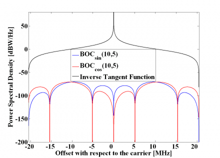
Figure 1: Power Spectral Density of Sine-phased, Cosine-phased and Inverse Tangent Function of BOC(10,5).

Credits
The information presented in this NAVIPEDIA’s article is an extract of the PhD work performed by Dr. Jose Ángel Ávila Rodríguez in the FAF University of Munich as part of his Doctoral Thesis “On Generalized Signal Waveforms for Satellite Navigation” presented in June 2008, Munich (Germany)