Detector based in code and carrier phase data: The Melbourne-Wübbena combination

Fundamentals
Title	Detector based in code and carrier phase data: The Melbourne-Wübbena combination
Author(s)	J. Sanz Subirana, J.M. Juan Zornoza and M. Hernández-Pajares, Technical University of Catalonia, Spain.
Level	Advanced
Year of Publication	2011

The Melbourne-Wübbena combination provides a noisy estimation of the wide-lane ambiguity [math]\displaystyle{ B_W }[/math], according to the following equation:

[math]\displaystyle{ B_W = \Phi_W - R_N= \lambda_W N_W +b_W+\varepsilon \qquad \mbox{(1)} }[/math]

where [math]\displaystyle{ N_W=N_1-N_2 }[/math] is the integer wide-lane ambiguity, [math]\displaystyle{ b_W }[/math] accounts for the satellite and receiver instrumental delays and [math]\displaystyle{ \varepsilon }[/math] is the measurement noise, including carrier phase and code multipath (see Combining pairs of signals and clock definition)

This combination has a double benefit: On one hand, the wide-lane combination has a larger wavelength [math]\displaystyle{ \lambda_W=c/(f_1-f_2) }[/math] than each signal individually, which leads to an enlarging of the ambiguity spacing . On the other hand, the measurement noise is reduced by the narrow-lane combination of code measurements , reducing the dispersion of values around the true bias.

A simple algorithm, but suitable to run in real-time, is presented as follows :

Algorithm description:

The detection is based on a real-time computation of mean and sigma values of the measurement test data [math]\displaystyle{ B_W }[/math]. A cycle-slip is declared when a measurement differs from the mean bias value over a predefined number of standard deviations ([math]\displaystyle{ S_{B_W} }[/math]) threshold (more details can be found in [Blewitt, 1990] .

Input data: Melbourne-Wübbena combination of [math]\displaystyle{ B_W }[/math] of code carrier phase.

Output: satellite (PRN), time, cycle-slip flag

For each epoch ([math]\displaystyle{ k }[/math])

For each tracked satellite ([math]\displaystyle{ s }[/math])

• Declare cycle-slip when data hole greater than [math]\displaystyle{ tol_{\Delta t} }[/math] (e.g., [math]\displaystyle{ 60\,s }[/math]).
• If no data hole larger than [math]\displaystyle{ tol_{\Delta t} }[/math], thence:
• Compare the measurement [math]\displaystyle{ B_W(s;k) }[/math] at the epoch [math]\displaystyle{ k }[/math] with the mean bias [math]\displaystyle{ m_{B_W}(s;k-1) }[/math] computed from the previous values. If the discrepancy is over a [math]\displaystyle{ threshod=K_{factor}*S_{B_W} }[/math] (e.g., [math]\displaystyle{ K_{factor}=4 }[/math]), declare cycle-slip.That is:

If [math]\displaystyle{ |B_W(s;k)-m_{B_W}(s;k-1)| \gt K_{factor} \,S_{B_W}(s;k-1) }[/math],

Thence, cycle-slip.

• Update the mean and sigma values according to the equations:

[math]\displaystyle{ \begin{array}{l} m_{B_W}(s;k)= \displaystyle \frac{k-1}{k} m_{B_W}(s;k-1) + \displaystyle \frac{1}{k} B_W(s;k)\\ \\[-0.3cm] S_{B_W}^2(s;k)= \displaystyle \frac{k-1}{k} S_{B_W}^2(s;k-1) + \displaystyle \frac{1}{k} {\left (B_W(s;k)- m_{B_W}(s;k-1) \right )^2} \end{array} \qquad \mbox{(2)} }[/math]

Note the [math]\displaystyle{ S_{B_W} }[/math] is initialised with an a priori [math]\displaystyle{ S_{0}=\lambda_w/2 }[/math].

• Reset algorithm after cycle slip.

End

End

Comments:

• The calculation of the mean is exact (over the [math]\displaystyle{ k=1,\dots,n,\dots }[/math] samples), while the computation of sigma is a good approximation ([math]\displaystyle{ O(1/k^2) }[/math]).

• A bottom, or bottom and upper, limit for the threshold can be set in order to prevent the test against unrealistic of noise estimates of [math]\displaystyle{ S_{B_W} }[/math].

• The mean bias estimate [math]\displaystyle{ m_{B_W} }[/math] can be highly affected by strong code multipath at the beginning of the data arch (due to low elevation raising satellites), but as the number of averaged samples increase, this estimation becomes more stable and robust. This improvement with the number of processed samples does not necessarily benefit to the [math]\displaystyle{ S_{B_W} }[/math] as an estimator of the data noise to define the detection threshold. Indeed, as the number of samples increase, the value of [math]\displaystyle{ S_{B_W}^2 }[/math] is being frozen, becoming more insensitive to the measurement noise variations. A solution to deal with this problem can be to compute a {\em moving sigma} (only for the [math]\displaystyle{ S_{B_W} }[/math], not [math]\displaystyle{ m_{B_W} }[/math]) over the last [math]\displaystyle{ N }[/math] sample window as in Examples of single frequency Cycle-Slip Detectors

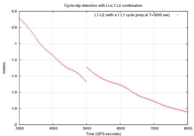
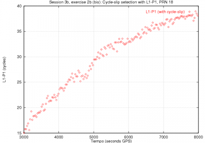
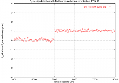
The effect of the ambiguity space widespread produced by the Melbourne-Wübbena combination is shown in next figure 2 and it is compared with the single frequency phase minus code combination (see Examples of single frequency Cycle-Slip Detectors as a reference. As in figure 1 of the Detector based in carrier phase data: The geometry-free combination, a jump of [math]\displaystyle{ 1 }[/math] cycle is introduced in the [math]\displaystyle{ \Phi_1 }[/math] carrier phase measurement at time [math]\displaystyle{ 5000 }[/math] seconds. This jump can not be identified from the [math]\displaystyle{ \Phi-R }[/math] combination shown in the left plot of figure 2 due to the receiver code noise and multipath, and to the ionospheric drift. On the contrary, it is clearly seen in the Melbourne-Wübbena combination plot shown at right of figure 2, which has a lower relative noise and it is not affected by the ionospheric refraction.

Figure 1: Effect of 1-cycle jump in GPS [math]\displaystyle{ \Phi_{L_1} }[/math] carrier phase signal on the ionosphere free combination. The horizontal axis is seconds of day. The vertical axis is in meters.

Figure 2: Effect of a 1-cycle jump in GPS [math]\displaystyle{ L_1 }[/math] signal in the [math]\displaystyle{ \Phi-R }[/math] (left) and Melbourne-Wübbena (right) combination (raw measurements without smoothing). Vertical axes are in cycles of [math]\displaystyle{ \lambda_1\simeq19\, cm }[/math] (left) and [math]\displaystyle{ \lambda_w\simeq86\,cm }[/math] (right).

frameless

frameless

The previous figure 2 shows a nice example of cycle-slip detection with the Melbourne-Wübbena combination, where the jump is well defined . Unfortunately, this is not the case in many occasions, being the detection threshold "fussier" due to the code receiver noise and multipath. This noise is smoothed by the filter averaging, i.e., by computing the mean bias [math]\displaystyle{ B_W }[/math], but still small jumps can escape to the detector in the first epochs following a filter reset.

Large code multipath, or even worse, undetected cycle-slips, at the beginning of the filter convergence, can propagate forward large errors, which can lead to a large [math]\displaystyle{ S_{B_W} }[/math] values, increasing the detection threshold ([math]\displaystyle{ K_{factor}*S_{B_W} }[/math]) and, thence, causing miss-detections. On the other hand, the use of small [math]\displaystyle{ K_{factor} }[/math] values to increase the detector sensibility can lead to a higher fault-detection probability.

References

- ^ [Blewitt, 1990] Blewitt, G., 1990. An automatic editing Algorithms for GPS data. Geophysical Research Letters. 17(3), pp. 199-202.