Tropospheric Delay

Fundamentals
Title	Tropospheric Delay
Author(s)	J. Sanz Subirana, J.M. Juan Zornoza and M. Hernández-Pajares, Technical University of Catalonia, Spain.
Level	Intermediate
Year of Publication	2011

Troposphere is the atmospheric layer placed between earth's surface and an altitude of about 60 kilometres.

The effect of the troposphere on the GNSS signals appears as an extra delay in the measurement of the signal traveling from the satellite to receiver. This delay depends on the temperature, pressure, humidity as well as the transmitter and receiver antennas location and, according to

[math]\displaystyle{ \Delta=\int_{_{\mbox{straight line}}}{(n-1)\,dl}\qquad\mbox{(1)} }[/math]

it can be written as:

[math]\displaystyle{ T=\int (n-1) \,dl =10^{-6}\int N \,dl \qquad\mbox{(2)} }[/math]

where [math]\displaystyle{ n }[/math] is the refractive index of air and [math]\displaystyle{ N }[/math] is the refractivity. The refractivity can be divided in hydrostatic, i.e., Dry gases (mainly N[math]\displaystyle{ _2 }[/math] and O[math]\displaystyle{ _2 }[/math]), and wet, i.e., Water vapour, components [math]\displaystyle{ N=N_{hydr}+N_{wet} }[/math].

Each of these components has different effects on GNSS signals. The main feature of the troposphere is that it is a non dispersive media with respect to electromagnetic waves up to 15GHz, i.e., the tropospheric effects are not frequency dependent for the GNSS signals. Thence, the carrier phase and code measurements are affected by the same delay.

An immediate consequence of being a non-frequency dependent delay is that the tropospheric refraction can not be removed by combinations of dual frequency measurements (as it is done with the ionosphere). Thence, the only way to mitigate tropospheric effect is to use models and/or to estimate it from observational data. Nevertheless, fortunately, most of the tropospheric refraction (about the 90%) comes from the predictable hydrostatic component [Leick, 1994]

A brief description on the atmosphere dry and wet component effects on the GNSS signals is given as follows:

• Hydrostatic component delay: It is caused by the dry gases present at the troposphere (78% N[math]\displaystyle{ _2 }[/math], 21% O[math]\displaystyle{ _2 }[/math], 0.9% Ar...). Its effect varies with local temperature and atmospheric pressure in quite a predictable manner, besides its variation is less that the 1% in a few hours. The error caused by this component is about 2.3 meters in the zenith direction and 10 meters for lower elevations ([math]\displaystyle{ 10^o }[/math] approximately).

• Wet component delay: it is caused by the water vapour and condensed water in form of clouds and, thence, it depends on weather conditions. The excess delay is small in this case, only some tens of centimetres, but this component varies faster than the hydrostatic component and a quite randomly way, being very difficult to model.

The dry atmosphere can be modeled from surface pressure and temperature using the laws of the ideal gases. The wet component is more unpredictable and difficult to model, thence for high precision navigation, this delay is estimated together with the coordinates.

The tropospheric delay depends on the signal path through the neutral atmosphere, and thence, can be modeled as a function of the satellite elevation angle. Due to the differences between the atmospheric profiles of the dry gases and water vapour it is better to use different mappings for the dry and wet components. Nevertheless, simple models as [RTCA-MOPS, 2006]use a common mapping for both components.

Several nominal tropospheric models are available in the literature, which differ on the assumptions made on the vertical profiles and mappings. Basically, they can be classified in two main groups: Geodetic-oriented or Navigation-oriented. The first group Sastamoinen, Hopfield, among others [Xu, 2007] are more accurate but generally more complex, and need surface meteorological data, being their accuracy affected by the quality of these data. The second group are less accurate, but meteorological data are not needed.

Example of Tropospheric model for Standard Point Positioning

The tropospheric model presented here is from [Collins, 1999]and it is the model adopted by the SBAS (WAAS, EGNOS...) systems [RTCA-MOPS, 2006]

In this case, there is a common mapping function for wet and dry troposphere:

[math]\displaystyle{ T(E)=(T_{z,dry}+T_{z,wet})\,M(E) \qquad\mbox{(3)} }[/math]

where [math]\displaystyle{ T_{z,dry} }[/math] and [math]\displaystyle{ T_{z,wet} }[/math] are calculated from the receiver's height and estimates of five meteorological parameters: pressure [[math]\displaystyle{ P }[/math] ([math]\displaystyle{ mbar }[/math])], temperature [[math]\displaystyle{ T }[/math] ([math]\displaystyle{ ^oK }[/math])], water vapour pressure [[math]\displaystyle{ e }[/math] ([math]\displaystyle{ mbar }[/math])], temperature "lapse" rate [[math]\displaystyle{ \beta }[/math] ([math]\displaystyle{ ^oK/m }[/math])] and water vapour "lapse rate" [[math]\displaystyle{ \lambda }[/math] (dimensionless)]. The obliquity factor [math]\displaystyle{ M(E) }[/math] is the [Black and Eisner, 1984] mapping:

[math]\displaystyle{ {M(E)=\frac{1.001}{\sqrt{0.002001+sin^2(E)}}} \qquad\mbox{(4)} }[/math]

which is valid for satellite elevation angles [math]\displaystyle{ E }[/math] over 5 degrees.

For a given receiver latitude ([math]\displaystyle{ \phi }[/math]) and Day-Of-Year [math]\displaystyle{ D }[/math] (i.e., from January [math]\displaystyle{ 1 }[/math]st), the value of each meteorological parameter is computed from the averaged meteorological parameters of table 1.

Indeed, each parameter value ([math]\displaystyle{ P }[/math], [math]\displaystyle{ T }[/math], [math]\displaystyle{ e }[/math], [math]\displaystyle{ \beta }[/math], [math]\displaystyle{ \lambda }[/math]) is computed as:

[math]\displaystyle{ \xi(\phi,D)=\xi_0(\phi)-\Delta\xi(\phi)\,\cos \left [\frac{2\pi(D-D_{min})}{365.25}\right] \qquad\mbox{(5)} }[/math]

where [math]\displaystyle{ D_{min}=28 }[/math] for northern latitudes and [math]\displaystyle{ D_{min}=211 }[/math] for southern latitudes. The [math]\displaystyle{ \xi_0(\phi) }[/math] and [math]\displaystyle{ \Delta\xi(\phi) }[/math] are the average and seasonal variation values at the receiver latitude ([math]\displaystyle{ \Phi }[/math]) linearly interpolated from table 1.

The Zero-altitude vertical delay terms [math]\displaystyle{ T_{z,dry} }[/math] and [math]\displaystyle{ T_{z,wet} }[/math] are given by:

[math]\displaystyle{ T_{z_0,dry}= \frac{10^{-6}\,k_1\, R_d\, P}{g_m}\;\;\; ; \qquad T_{z_0,wet}= \frac{10^{-6}\,k_2\, R_d}{(\lambda +1)\,g_m-\beta\, R_d}\frac{e}{T} \qquad\mbox{(6)} }[/math]

The vertical delay [math]\displaystyle{ T_{z,dry} }[/math] and [math]\displaystyle{ T_{z,wet} }[/math] at the receiver height [math]\displaystyle{ H }[/math] are calculated as:

[math]\displaystyle{ T_{z,dry}= \left [ 1-\frac{\beta \,H}{T} \right ]^{\frac{g}{R_d\,\beta}} \cdot T_{z_0,dry}\;\;\; ; \qquad T_{z,wet}=\left [ 1-\frac{\beta \,H}{T} \right ]^{\frac{(\lambda +1)g}{R_d\,\beta}-1}\cdot T_{z_0,wet} \qquad\mbox{(7)} }[/math]

where [math]\displaystyle{ H }[/math] is the height above the mean-sea-level, in meters, [math]\displaystyle{ k_1= 77.604\, K/mbar }[/math], [math]\displaystyle{ k_2= 382000\, K^2/mbar }[/math], [math]\displaystyle{ R_d = 287.054\, J/Kg/K }[/math], and [math]\displaystyle{ g_m = 9.784\, m/s^2 }[/math].

Figure 1 illustrates with an example the values of the tropospheric delay and the effect of neglecting such delays in standard point positioning for the horizontal and vertical error components.

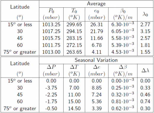Table 1: Meteorological parameters for the tropospheric delay. Parameters for latitudes [math]\displaystyle{ 15^o \lt |\Phi| \lt 75^o }[/math], must be linearly interpolated between values for the two closest latitudes [math]\displaystyle{ [\Phi_i,\Phi_{i+1}] }[/math]. Parameters above [math]\displaystyle{ |\phi|\leq 15^o }[/math] and [math]\displaystyle{ |\phi| \geq 75^o }[/math] are taken directly from the table.

Figure 1: Tropospheric correction: Range and position domain effect

frameless	frameless
frameless	First row shows the horizontal (left) and vertical (right) positioning error using (blue) or not using (red) the tropospheric correction (equation 3). The variation in range is shown in the second row at left

Example of Tropospheric model for Precise Point Positioning

The example presented here is one of the tropospheric models implemented in the GIPSY-OASIS II software, which does not require any surface meteorological data. This model uses the Mapping of Niell, that considers different obliquity factors for the wet and dry components:

[math]\displaystyle{ T(E)=T_{z,dry}\cdot M_{dry}(E)+T_{z,wet}\cdot M_{wet}(E) \qquad\mbox{(8)} }[/math]

In this implementation, the wet tropospheric delay is estimated by the navigation filter together with the receiver position. This approach allows a huge simplification of the model for the vertical delays, which nominal values are:

[math]\displaystyle{ \begin{array}{l} T_{z,dry}= a\; e^{-b\; H}\\ T_{z,wet}= T_{z_0,wet}+\Delta T_{z,wet} \end{array} \qquad\mbox{(9)} }[/math]

where [math]\displaystyle{ a=2.3 \,m }[/math], [math]\displaystyle{ b=0.116\cdot 10^{-3} }[/math], and [math]\displaystyle{ H }[/math] is the height over the sea level, in meters. [math]\displaystyle{ T_{z_0,wet}=0.1\, m }[/math] and [math]\displaystyle{ \Delta T_{z,wet} }[/math] is estimated as a random-walk process (typically [math]\displaystyle{ 1\;cm^2/h }[/math] of process noise) in the navigation --Kalman-- filter together with the coordinates, and other parameters (see Linear observation model for PPP. The accuracy of the [math]\displaystyle{ \Delta T_{z,wet} }[/math] estimates in static positioning is at the centimetre level.

Figure 2 shows a comparison of Zenith Tropospheric Delay (ZTD) estimate (static PPP) with the IGS determination.

Figure 2: Comparison of ZTD (PPP) estimate with IGS determination.

Further information about the tropospheric correction model defined in GALILEO can be found here

References

- ^ [Leick, 1994] Leick, A., 1994. GPS Satellite Surveying. Wiley-Interscience Publication, USA.
- ^ a b [RTCA-MOPS, 2006] RTCA-MOPS, 2006. Minimum Operational Performance Standards for Global Positioning System / Wide Area Augmentation System Airborne Equipment.rtca document 229-c.
- ^ [Xu, 2007] Xu, G., 2007. GPS: theory, algorithms, and applications. Springer-Verlar, Germany.
- ^ [Collins, 1999] Collins, J., 1999. Assessment and Development of a Tropospheric Delay Model for Aircraft Users of the Global Positioning System. M.Sc.E. thesis, Department of Geodesy and Geomatics Engineering Technical Report No. 203, University of New Brunswick, Fredericton, New Brunswick, Canada.
- ^ [Black and Eisner, 1984] Black, H. and Eisner, A., 1984. Correcting satellite Doppler data for tropospheric effects. Journal of Geophysical Research. 89, pp. 2616{2626.