If you wish to contribute or participate in the discussions about articles you are invited to contact the Editor
Transformations between Time Systems: Difference between revisions
Jaume.Sanz (talk | contribs) No edit summary |
Carlos.Lopez (talk | contribs) No edit summary |
||
| Line 4: | Line 4: | ||
|Level=Intermediate | |Level=Intermediate | ||
|YearOfPublication=2011 | |YearOfPublication=2011 | ||
|Title={{PAGENAME}} | |Title={{PAGENAME}} | ||
}} | }} | ||
Revision as of 11:42, 23 February 2012
| Fundamentals | |
|---|---|
| Title | Transformations between Time Systems |
| Author(s) | J. Sanz Subirana, J.M. Juan Zornoza and M. Hernández-Pajares, Technical University of Catalonia, Spain. |
| Level | Intermediate |
| Year of Publication | 2011 |

As a summary for further explanations, in Figure 1 can be seen a layout of the different time scales.
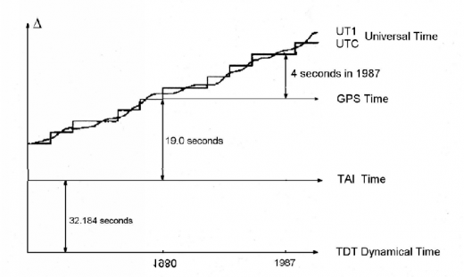 Figure 1: Time flowing (from [Seeber, 1993] [1]).

Figure 2 summarises the relationship between different times described before. As showed in this graphic most of the times are computed quite straightforward only by applying a constant offset. The next sections explain the procedures to transform one time type into another.

GNSS – TAI
As said before, the difference between GPS time (GPST) and TAI times is always a constant offset of 19 seconds. Thus:
- [math]\displaystyle{ TAI=GPST+19.000\ seconds \qquad \mbox{(1)} }[/math]
GLONASS time is synchronised to UTC, with a [math]\displaystyle{ 3 }[/math] hours shift due to the difference between Moscow time and GMT. Thence,
- [math]\displaystyle{ TAI=GLONASST-3\,hours+Leap\ Second \qquad \mbox{(2)} }[/math]
TAI – UTC
The difference between these times is given by the accumulated Leap Seconds. These Leap Seconds are provided by the International Earth Rotation Service (IERS). The IGS centres provide files with the earth's rotation parameters and time information, which are actualised periodically (see http://acc.igs.org).
- [math]\displaystyle{ UTC=TAI-Leap\ Seconds \qquad \mbox{(3)} }[/math]
With the introduction of the Leap Second, the UTC time (which is an atomic time) does not differ from the earth's rotational time (UT1) by more than [math]\displaystyle{ 0.9 }[/math] seconds.
TAI - UT1
An a priory UT1 [math]\displaystyle{ \left( \widehat{UT1} \right ) }[/math] can be computed by:
- [math]\displaystyle{ \widehat{UT1}=UT1R+\Delta UT1 \qquad \mbox{(4)} }[/math]
- Thence
- [math]\displaystyle{ TAI-\widehat{UT1}=[TAI-UT1R]-\Delta UT1 \qquad \mbox{(5)} }[/math]
where UT1R is an smoothed a priory measurement of the earth's orientation for which the short period ([math]\displaystyle{ t\lt 35 }[/math] days) tidal effects have been removed before smoothing [Webb and Zumberge, 1993] [2].
The TAI-UT1R or UTC-UT1R is provided in the Earth's Rotation Parameters files [footnotes 1].
According to [Yoder et al., 1981] [3] the periodic variations of UT1 due to the tidal deformations of the polar moment of inertia can be given by:
- [math]\displaystyle{ \Delta UT1=\sum_{i=1}^N\left[ A_i \; \sin \left(\sum_{j=1}^5 k_{ij}\; \alpha _j\right) \right] \qquad \mbox{(6)} }[/math]
The number [math]\displaystyle{ N }[/math] is chosen to include all terms with a period less than [math]\displaystyle{ 35 }[/math] days. The [math]\displaystyle{ \alpha _j }[/math] are the functions of time given by equations (6) to (10) in ICRF to CEP.
- [math]\displaystyle{ \alpha_1=l=485\,866_{\cdot}^{\prime \prime}733+(1\,325^r+715\,922_{\cdot}^{\prime \prime}633)\; T+31_{\cdot}^{\prime \prime}310\; T^2+0_{\cdot}^{\prime \prime}064\; T^3 \qquad \mbox{(7)} }[/math]
- [math]\displaystyle{ \alpha_2=l^{\prime }=1\,287\,099_{\cdot}^{\prime \prime}804+(99^r+1\,292\,581_{\cdot}^{\prime \prime}224)\; T-0_{\cdot}^{\prime \prime}577\; T^2-0_{\cdot}^{\prime \prime}012\; T^3 \qquad \mbox{(8)} }[/math]
- [math]\displaystyle{ \alpha_3=F=335\,778_{\cdot}^{\prime \prime}877+(1342^r+295\,263_{\cdot}^{\prime \prime}137)\; T-13_{\cdot}^{\prime \prime}257\; T^2+0_{\cdot}^{\prime \prime}011\; T^3 \qquad \mbox{(9)} }[/math]
- [math]\displaystyle{ \alpha_4=D=1\,072\,261_{\cdot}^{\prime \prime}307+(1\,236^r+1\,105\,601_{\cdot}^{\prime \prime}328)\; T-6_{\cdot}^{\prime \prime}891\; T^2+0_{\cdot}^{\prime \prime}019\; T^3 \qquad \mbox{(10)} }[/math]
- [math]\displaystyle{ \alpha_5=\Omega =450\,160_{\cdot}^{\prime \prime}280-(5^r+482\,890_{\cdot}^{\prime \prime}539)\; T+7_{\cdot}^{\prime \prime}455\; T^2+0_{\cdot}^{\prime \prime}008\; T^3 \qquad \mbox{(11)} }[/math]
The parameters [math]\displaystyle{ A_i }[/math], [math]\displaystyle{ k_{ij} }[/math] are given in Table 1 of article ICRF to CEP for periods up to [math]\displaystyle{ 41 }[/math] days. A table with periods up to [math]\displaystyle{ 18.6 }[/math] years ([math]\displaystyle{ 62 }[/math] terms) based on [Yoder et al., 1981] is available in http://hpiers.obspm.fr/eop-pc/models/UT1/UT1R_tab.html. An extended model with "[math]\displaystyle{ \sin }[/math]" and "[math]\displaystyle{ \cos }[/math]" terms is given in the IERS03 conventions, (see [Denis et al., 2004][4], page 92) with the associated table of coefficients.
UT0, UT1, UT2
As commented before, UT0, UT1 and UT2 are Universal Times linked to the earth's rotation.
The UT1 and UT0 are related by the following expression, where [math]\displaystyle{ \Delta l }[/math] is a correction of longitude due to the effect of polar motion:
- [math]\displaystyle{ \begin{array}{c} UT1=UT0+\Delta l \end{array} \qquad \mbox{(12)} }[/math]
- where:
- [math]\displaystyle{ \begin{array}{c} \Delta l=\frac{1^{s}}{15}\;(x_p\; \sin \lambda -y_p\; \cos \lambda)\; \tan \varphi \end{array} \qquad \mbox{(13)} }[/math]
In this expression [math]\displaystyle{ x_p }[/math] and [math]\displaystyle{ y_p }[/math] are the instantaneous pole coordinates (see figure (2) in CEP to ITRF) while [math]\displaystyle{ \lambda }[/math] and [math]\displaystyle{ \varphi }[/math] are the site latitude and longitude respectively [footnotes 2]. With this rotation axis correction the pole movement in longitude ([math]\displaystyle{ \Delta l }[/math]) is removed and one passes from the instantaneous pole (CEP) to the Conventional Terrestrial Pole (CTP), see figure (1) in Transforming Celestial to Terrestrial Frames, at right side.
UT2 is obtained correcting UT1 by the periodic seasonal variation on the earth rotation:
- [math]\displaystyle{ UT2=UT1+\Delta S \qquad \mbox{(14)} }[/math]
where:
- [math]\displaystyle{ \Delta S=0^s_{\cdot}022\; \sin{2\pi t}-0^s_{\cdot}120\; \cos{2\pi t}-0^s_{\cdot}0060\sin{4\pi t}+0^s_{\cdot}0070\; \cos{4\pi t} \qquad \mbox{(15)} }[/math]
with [math]\displaystyle{ \Delta S }[/math] in seconds and [math]\displaystyle{ t }[/math] being the date in Besselian years:
- [math]\displaystyle{ t=2000.00+\frac{MJD-51\,544.03}{365.2422} \qquad \mbox{(16)} }[/math]
TAI - TDT, TCG, TT
As commented before, after the IAU resolution of 1991, the TDT is substituted by the Geocentric Coordinate Time (TCG) and Terrestrial Time (TT), where TT corresponds to the TDT in the former definition (before 1991). Thence
- [math]\displaystyle{ TDT\equiv TT=TAI+32.184\ seconds \qquad \mbox{(17)} }[/math]
where TAI is a realization of TT, apart from a constant offset of [math]\displaystyle{ 32.184 }[/math] seconds.
On the other hand, TCG and TT are related by [Denis et al., 2004]:
- [math]\displaystyle{ \begin{array}{c} TCG-TT=L_G\;(MJD-43\,144.0)\; 86\,400\,s\\ \mbox{with}\\ L_G=6.969290134\;10^{-10} \end{array} \qquad \mbox{(18)} }[/math]
TDT - TDB, TCB
The relationship between these times is given by the equation:
- [math]\displaystyle{ \begin{array}{c} TDB=TDT+0^s_{\cdot}001658 \; \sin(g+0.0167 \; \sin g ) \\ \\ g=\displaystyle{\frac{2 \; \pi \; (357^o_{\cdot}528+35\,999^o_{\cdot}050 \; T)}{360^{o}}} \end{array} \qquad \mbox{(19)} }[/math]
where T is in centuries from J2000 of TDT [footnotes 3]:
- [math]\displaystyle{ Centuries=\frac{Julian\ date-2\,451\,545.0}{36\,525} \qquad \mbox{(20)} }[/math]
As in the case of TDT, after the IAU resolution of 1991, the TBD is substituted by Barycentric Coordinate Time (TCB), which is related with TDB by [Denis et al., 2004]:
- [math]\displaystyle{ \begin{array}{c} TCB-TDT=L_B\;(MJD-43\,144.0)\; 86\,400\,s+P_0\\ \mbox{with}\\ L_B=1.55051976772\;10^{-8},\mbox{ and }P_0\simeq 6.55\, 10^{-5}s. \end{array} \qquad \mbox{(21)} }[/math]
Notes
- ^ Earth orientation parameters and time information are provided in different servers and with different format files: "erp" files, the GIPSY format "TPNML" and "tpeo.nml" files. See ftp://igscb.jpl.nasa.gov/pub/product/iers/ or http://acc.igs.org/, or the JPL sites: ftp://sideshow.jpl.nasa.gov/pub/gipsy_products/2009/orbits/, ftp://sideshow.jpl.nasa.gov/pub/gipsy_products/RapidService/orbits/.
- ^ The [math]\displaystyle{ x_p }[/math] and [math]\displaystyle{ y_p }[/math] pole displacements are given in the previously mentioned Earth Rotation Parameters files (e.g., the JPL TPNML files).
- ^ To obtain TDT from TDB, the T can be taken as centuries from J2000 of TDT, without incurring in significant error.
References
- ^ [Seeber, 1993] Seeber, G., 1993. Satellite Geodesy: Foundations, Methods, and Applications. Walter de Gruyter & Co., Berlin, Germany.
- ^ [Webb and Zumberge, 1993] Webb, F. and Zumberge, J., 1993. An Introduction to GIPSY/OASIS-II. Jet Propulsion Laboratory, JPL, 4800 Oak Grove Drive, Pasadena, CA 91109.
- ^ [Yoder et al., 1981] Yoder, C., Williams, J. and Parke, M., 1981. Tidal Variations of Earth Rotation. Journal of Geophysical Research. pp. 881-891.
- ^ [Denis et al., 2004] Denis, D., McCarthy and Petit, G., 2004. IERS Conventions (2003). IERS Technical Note 32. IERS Convention Center, Frankfurt am Main.