If you wish to contribute or participate in the discussions about articles you are invited to contact the Editor
Detector based in carrier phase data: The geometry-free combination
| Fundamentals | |
|---|---|
| Title | Detector based in carrier phase data: The geometry-free combination |
| Author(s) | J. Sanz Subirana, J.M. Juan Zornoza and M. Hernández-Pajares, Technical University of Catalonia, Spain. |
| Level | Advanced |
| Year of Publication | 2011 |
With two frequency signals it is possible to make the carrier phase geometry free combination, in order to remove the geometry, including clocks, and all non dispersive effects in the signal. This very precise (with very low noise) test signal performs as a smooth function, driven by the ionospheric refraction, with very few changes between closely epochs. Indeed, although, for instance, the jump produced by a simultaneous 1-cycle slip in both signal components is smaller in this combination than in the original signals [footnotes 1], it can provide a reliable detection, also for small jumps.
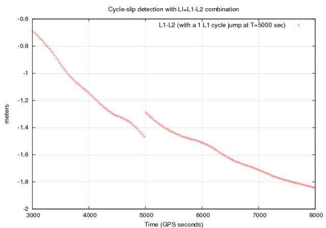
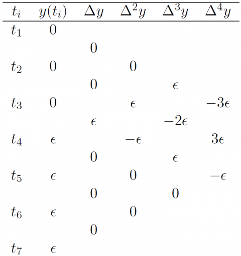
The easiest way to build a cycle-slip detector is just to consider the differences in time of consecutive samples (see figure 1). A refinement of this procedure is the use of the n-order differences to take benefit of the jumps amplitude enlargement produced by the differencing process (see Table 1 from [Hofmann-Wellenhof et al., 2008] [1]).
This approach allows making a reasonable enough detector for many applications. Nevertheless, it must be taken into account that as the jumps are enlarged also the signal noise (i.e., signal instabilities) is amplified, which can lead to false detections in some scenarios (for instance with low signal to noise ratios, ionospheric scintillation…).
A way to mitigate the impact of these effects is to use a low order polynomial fit, reducing the test signal noise. This concept is the basis of the detector's example presented as follows:
Algorithm description:
The detection is based on fitting a second degree polynomial over a sliding window of [math]\displaystyle{ N_I }[/math] samples (e.g., [math]\displaystyle{ N_I=10 }[/math]). The predicted value from this polynomial is compared with the observed value to detect the cycle-slip. As the geometry-free combination is affected by the ionospheric refraction, a sampling rate dependent threshold is considered.
Input data: Geometry-free combination of carrier phase measurements.
[math]\displaystyle{ \Phi_{L_I}(s;k)=\Phi_1(s;k)-\Phi_2(s;k) }[/math]
Output: satellite (PRN), time, cycle-slip flag
- For each epoch ([math]\displaystyle{ k }[/math])
- For each tracked satellite ([math]\displaystyle{ s }[/math])
- Declare cycle-slip when data hole greater than [math]\displaystyle{ tol_{\Delta t} }[/math] [footnotes 2]
- Fit a second degree polynomial [math]\displaystyle{ P(s;x) }[/math] to the previous values (after the last cycle-slip)[footnotes 3] [math]\displaystyle{ \Phi_{L_I}(s;k-N_I),\dots,\Phi_{L_I}(s;k-1)] }[/math].
- Compare the measured [math]\displaystyle{ \Phi_{L_I}(s;k) }[/math] and the predicted value [math]\displaystyle{ P(s;k) }[/math] at the epoch [math]\displaystyle{ k }[/math]. If the discrepancy is over a given [math]\displaystyle{ threshod }[/math], thence declare cycle-slip. That is:
- If [math]\displaystyle{ |\Phi_{L_I}(s;k)-P(s;k)| \gt Threshold }[/math],
- Thence, cycle-slip.
- Reset algorithm after cycle slip.
- End
- For each tracked satellite ([math]\displaystyle{ s }[/math])
- End
Comments:
The relative variation between two consecutive epochs [math]\displaystyle{ t_1 }[/math] and [math]\displaystyle{ t_2 }[/math] depends of the elapsed time interval in between (i.e., [math]\displaystyle{ \Delta t=t_2-t_1 }[/math]), due to the ionospheric refraction variation. Thence, a [math]\displaystyle{ \Delta t }[/math]-dependent threshold is recommended to account for the measurement sampling rate. For instance: [math]\displaystyle{ Threshod=a_0-a_1 \, \exp(-\Delta t/T_0) }[/math] can be used.
Notice that [math]\displaystyle{ a_0 }[/math] is the maximum threshold. On the other hand, taking for instance [math]\displaystyle{ a_1=a_0/2 }[/math], thence the threshold is [math]\displaystyle{ a_0 [1-\frac{e^{-\Delta t/T_0}}{2}] }[/math], which, for [math]\displaystyle{ T_0=60 }[/math] seconds, corresponds to about [math]\displaystyle{ a_0/2 }[/math] for [math]\displaystyle{ 1 }[/math] second sampling rate and about [math]\displaystyle{ 2a_0/3 }[/math] for [math]\displaystyle{ 30 }[/math] seconds sampling rate data. In this way, if [math]\displaystyle{ a_0 }[/math] is set as [math]\displaystyle{ a_0=\frac{3}{2}(\lambda_2-\lambda_1) }[/math], the minimum detectable jump, between two contiguous measurements, will be [math]\displaystyle{ \frac{3}{4}(\lambda_2-\lambda_1) }[/math] or [math]\displaystyle{ \lambda_2-\lambda_1 }[/math] for [math]\displaystyle{ 1 }[/math] second or [math]\displaystyle{ 30 }[/math] seconds sampling rate, respectively [footnotes 4]
Notes
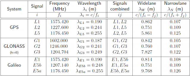
- ^ For GPS signals, this jump is [math]\displaystyle{ \lambda_2-\lambda_1=5.4\,cm }[/math], which is about 3-4 times shorter than [math]\displaystyle{ \lambda_1=19.0\,cm }[/math] or [math]\displaystyle{ \lambda_2=24.4\,cm }[/math] (see Table 2)
- ^ For instance, 60 seconds.
- ^ A simplest approach is construct a Lagrange interpolating polynomial with the last three values. This would be equivalent to consider the 3rd-order differences in time of consecutive samples (i.e., [math]\displaystyle{ \Delta^3 P_2(t)\equiv 0 }[/math]).
- ^ From Figure 2 notice that [math]\displaystyle{ \lambda_2-\lambda_1 }[/math] is the jump produced on the geometry-free combination [math]\displaystyle{ \Phi_I }[/math] when a jump of [math]\displaystyle{ 1 }[/math] cycle occurs simultaneously in both carriers. This jump, for instance, for the GPS L1, L2 signals is [math]\displaystyle{ \lambda_{L2}-\lambda_{L1}=5.4\, cm }[/math] (see table 2)
References
- ^ [Hofmann-Wellenhof et al., 2008] Hofmann-Wellenhof, B., Lichtenegger, H.,K. and Wasle, E., 2008. GNSS - Global Navigation Satellite Systems.. Springer-Verlag, Wien, Austria.


