If you wish to contribute or participate in the discussions about articles you are invited to contact the Editor
Combining pairs of signals and clock definition: Difference between revisions
Jaume.Sanz (talk | contribs) No edit summary |
Jaume.Sanz (talk | contribs) No edit summary |
||
| Line 175: | Line 175: | ||
</math> | </math> | ||
Once the <math>I+K_{21}</math> sum is computed, the DCBs (<math>K_{21}</math>) can be | Once the <math>I+K_{21}</math> sum is computed, the DCBs (<math>K_{21}</math>) can be decorrelated from the ionospheric refraction (<math>I</math>) using a geometrical description of the ionosphere, i.e., describing the satellite-receiver ray ionospheric sounding, due to the satellite motion along its path. In this way, the accuracy of the ionosphere and DCBs determinations mostly relies on the geometrical model used to describe the ionosphere (i.e., one layer model or two layers voxel model [Hernandez-Pajares et al., 1999]). | ||
==References== | ==References== | ||
Revision as of 20:01, 4 February 2013
| Fundamentals | |
|---|---|
| Title | Combining pairs of signals and clock definition |
| Author(s) | J. Sanz Subirana, J.M. Juan Zornoza and M. Hernández-Pajares, Technical University of Catalonia, Spain. |
| Level | Advanced |
| Year of Publication | 2011 |

Before starting to apply the equations to the code and phase measurements, some arrangement will be done to the expressions
- [math]\displaystyle{ R_{_P}=\rho+c(dt_r-dt^s)+T+\alpha_f\,STEC+K_{P,r}-{K_P}^s+\mathcal{M}_P+\varepsilon_{_P} \qquad \mbox{(1)} }[/math]
- and
- [math]\displaystyle{ \Phi_L=\rho+c(dt_r-dt^s)+T-\alpha_f \, STEC+k_{L,r}-{k_L}^s+\lambda_L\,N_L+\lambda_L \,w+m_L+\epsilon_{_L} \qquad \mbox{(2)} }[/math]
in order to refer the clocks to the code ionosphere-free combination ([math]\displaystyle{ R_{_{PC}} }[/math]):
Defining a new clock [math]\displaystyle{ \delta t }[/math] as:
- [math]\displaystyle{ c\,\delta t= c\,dt+K_C~~,~~~\mbox{where}~~ K_C=\frac{f_1^2K_1-f_2^2K_2}{f_1^2-f_2^2} \qquad \mbox{(3)} }[/math]
it is not difficult to demonstrate that:
- [math]\displaystyle{ \begin{array}{c} c\,dt+K_1= c\,\delta t+\tilde{\alpha_1} (K_2-K_1)\\ c\,dt+K_2= c\,\delta t+\tilde{\alpha_2} (K_2-K_1) \end{array} \qquad \mbox{(4)} }[/math]
- with
- [math]\displaystyle{ \qquad \mbox{(5)} }[/math]


- where [math]\displaystyle{ dt }[/math], [math]\displaystyle{ \delta t }[/math], [math]\displaystyle{ K_1 }[/math], [math]\displaystyle{ K_2 }[/math] stand for either the satellite or the receiver clocks, and their instrumental delays.
The [math]\displaystyle{ K_2-K_1 }[/math] is the interfrequency bias between the code instrumental delays at the frequencies [math]\displaystyle{ f_1 }[/math] and [math]\displaystyle{ f_2 }[/math], also called Differential Code Biases (DCB). Let's do:
- [math]\displaystyle{ K_{21} \equiv K_2-K_1 \qquad \mbox{(6)} }[/math]
Notice that a different DCB would affect satellites and receivers. That is, the [math]\displaystyle{ K_{21,r} }[/math] receiver DCB is defined when applying [math]\displaystyle{ K_{1,r} }[/math] and [math]\displaystyle{ K_{2,r} }[/math] to the expression (4), and the [math]\displaystyle{ K_{21}^s }[/math] satellite DCB is defined when applying [math]\displaystyle{ K_1^s }[/math] and [math]\displaystyle{ K_2^s }[/math]. In order to simplify the notation, hereafter we will use [math]\displaystyle{ K_{21} \equiv K_{21,r}-K_{21}^s }[/math]. In the same way, we will use [math]\displaystyle{ K_i\equiv K_{i,r}-K_{i}^s }[/math], or [math]\displaystyle{ k_i\equiv k_{i,r}-k_{i}^s }[/math], for the code and phase instrumental delays corresponding to frequency [math]\displaystyle{ f_i }[/math].
The DCBs of the satellites are broadcast in the GNSS navigation messages as the TGD, (see Instrumental Delay). For instance, [math]\displaystyle{ TGD_{P1}=-\tilde{\alpha}_{1} K_{P21}^s }[/math] is broadcast in the legacy GPS message for the [math]\displaystyle{ P2-P1 }[/math] code interfrequency bias (see GPS Signal Plan), and the DCBs between the codes on frequencies [math]\displaystyle{ E1,E5a }[/math], and on frequencies [math]\displaystyle{ E5b,E1 }[/math], are broadcast in the Galileo F/NAV and I/NAV messages, respectively (see article GALILEO Signal Plan). IGS also provides DCBs for the GPS satellites and reference station receivers. These products match the IONEX TEC maps [footnotes 1] and the precise satellite orbits and clocks (see article Precise GNSS Satellite Coordinates Computation), which always refer to the code ionosphere-free combination [math]\displaystyle{ R_{_{PC}} }[/math].
Naming [math]\displaystyle{ I }[/math] the ionospheric delay in the geometry free combination:
- [math]\displaystyle{ I\equiv(\alpha_2-\alpha_1)\,STEC=\frac{40.3(f^2_1- f^2_2)}{f^2_1 f^2_2}10^{16}\,STEC \;\;\; (\mbox{units: }m_{\mbox{delay}_{(\Phi_1-\Phi_2)}}) \qquad \mbox{(6)} }[/math]
and substituting the expressions (4) in (1) and (2), it follows [footnotes 2]:
- [math]\displaystyle{ R_{_1}=\rho+c(\delta t_r-\delta t^s)+T+\tilde{\alpha_1}(I+K_{21})+\mathcal{M}_1+\varepsilon_1 \qquad \mbox{(7)} }[/math]
- [math]\displaystyle{ \Phi_{_1}=\rho+c(\delta t_r-\delta t^s)+T- \tilde{\alpha_1}(I+K_{21})+b_1+\lambda_1\,N_1+\lambda_1 w+m_1+\epsilon_1 \qquad \mbox{(8)} }[/math]
where [math]\displaystyle{ b_1=k_1-K_1+2\tilde{\alpha_1} K_{21} }[/math] is a frequency-dependent bias.
Notice that, as with the code instrumental delay, the carrier phase bias [math]\displaystyle{ b }[/math] can be split in two different terms, associated to the receiver and to the satellite. That is: [math]\displaystyle{ b_1=b_{1,r}-b_1^s }[/math].
Comment: At first glance it could be surprising to see the ‘code DCBs’ (i.e. [math]\displaystyle{ K_{21} }[/math] ) included in the equation of carrier phase measurements, joining the ionospheric term. Nevertheless, as will be shown next, it provides closed expressions for the different combinations of measurements, where the ionospheric term always joins the DCB as ‘[math]\displaystyle{ I +K_{21} }[/math] ’, with a frequency- dependent scale factor, see the equations below. In this way, combinations removing the ionosphere, such as MW, will also be free from DCBs. On the other hand, as the carrier measurement contains an unknown bias, it can be redefined without loss of generality to include such a term. See remarks and additional comments below.
Replacing the expressions of [math]\displaystyle{ R_i }[/math] and [math]\displaystyle{ \Phi_i }[/math], [math]\displaystyle{ i=1,2 }[/math] in the definitions
- [math]\displaystyle{ \Phi_{_{LI}}=\Phi_{_{L1}}-\Phi_{_{L2}}~~~~~;~~~~~ R_{_{PI}}=R_{_{P2}}-R_{_{P1}} \mbox{(9)} }[/math]
- to
- [math]\displaystyle{ \Phi_{_{LN}}=\frac{f_1\;\Phi_{_{L1}}+f_2\;\Phi_{_{L2}}}{f_1+f_2}~~~~~;~~~~~ R_{_{PN}}=\frac{f_1\;R_{_{P1}}+f_2\;R_{_{P2}}}{f_1+f_2} \qquad \mbox{(10)} }[/math]
the following expressions are found (see article Combination of GNSS Measurements) :
Remark: The Antenna Phase Centre (APC) effect is neglected here for simplicity (see article Antenna Phase Centre).


- [math]\displaystyle{ \qquad \mbox{(11)} }[/math]

The effect of a jump in the integer ambiguities is given by the next equations:

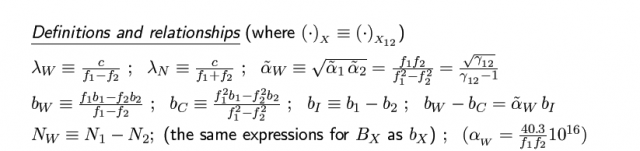
The different wavelengths for the wide-lanes and narrow-lanes combinations of frequencies in GPS, GLONASS (only channel [math]\displaystyle{ k=0 }[/math] is shown) and Galileo, as well as the values for the associated parameters, are given in the next tables:


Remarks on the previous equations:
- Although, for simplicity, the previous equations (11) are written in terms of two signals at frequencies [math]\displaystyle{ f_1 }[/math] and [math]\displaystyle{ f_2 }[/math], they are valid for any pair of frequencies [math]\displaystyle{ f_k }[/math] and [math]\displaystyle{ f_m }[/math] (see table 1).
- The code DCBs have been included in the equations of carrier phase measurements, joining the ionospheric term, to provide a closed expression (see the advanced comments below). Nevertheless, they could be included in the unknown bias [math]\displaystyle{ B_{_\Box} }[/math]. That is: [math]\displaystyle{ -\tilde{\alpha}_{_\Box}(I+K_{21})+B_{_\Box} \equiv \tilde{\alpha}_{_\Box} I +\hat{B}_{_\Box} }[/math]
- Notice that the wind-up term does not appear in the wide-lane carrier phase combination. This is because the signals are subtracted in cycles, see equation (2). That is, [math]\displaystyle{ \Phi_W=\frac{f_1 \Phi_1 -f_2 \Phi_2}{f_1 -f_2}=c\,\frac{\phi_1-\phi_2}{f_1-f_2} }[/math], and both signals are affected by the same fraction of cycle by the wind-up.
- The GRAPHIC combination [Yunck, 1993] [1] provides a ionosphere-free single frequency measurement with reduced noise (half than the code noise, see Receiver noise), but it contains the unknown ambiguity of the carrier phase. This combination is used, for instance, for GPS single-frequency orbit determination for Low Earth Orbiting (LEO) satellites, see for instance, [Montenbruck and Ramos-Bosch, 2007] [2], [Hernandez-Pajares et al., 1999] [3]
- Final Remark: The equations (11) are based in the redefinition of clock to cancel out the instrumental code delays in the ionosphere-free combination of codes [math]\displaystyle{ R_{_{PC}} }[/math].
Additional comments on the equations
A brief discussion on some issues related with the previous equations is provided to clarify their content and meaning.
Code based positioning The GNSS satellites broadcast in their navigation messages ephemeris and satellite clock information linked to the code ionosphere-free combination (PC). In this way, dual frequency users can navigate with the ionosphere-free combination, without needing either ionospheric corrections or DCBs. In the case of the legacy GPS navigation message, such DCBs correspond to the P1-P2.
For single frequency users, the navigation message provides the parameters of a ionospheric model together with the associated TGDs (see article Instrumental Delay).
Carrier phase based positioning (Advanced comments)
Thanks to the (satellite and receiver) clock re-definition (from expression 3), the ionosphere free combination of code measurements is free from DCBs (either for satellite or receivers). But this is not the case for the carrier phase measurements, which still contain the real bias [math]\displaystyle{ b_C=b_{C,rec}+b_C^{sat} }[/math] because the clocks have been referred to the code measurements.
Nevertheless, this carrier phase bias [math]\displaystyle{ b_C }[/math] is not a problem for carrier-phase based positioning techniques like the Precise Point Positioning (PPP) presented in article Code and Carrier Based Positioning (PPP), because it is assimilated in the unknown ambiguity when it is estimated by the Kalman Filter as a real number, i.e., floating the ambiguities.
It neither affects the ambiguity fixing in differential positioning techniques like Real Time Kinematics (RTK), because any remaining bias cancels out when forming the double differences between satellites and receivers [math]\displaystyle{ \nabla \Delta }[/math], remaining only the integer part of the ambiguities ([math]\displaystyle{ \nabla \Delta B_i= \nabla \Delta N_i }[/math], [math]\displaystyle{ i=1,2 }[/math]), see article Double differenced ambiguity fixing). Nevertheless, this bias (fractional part of the ambiguities) must be considered if the ambiguities are tried to be fixed in undifferenced mode, i.e., Undifferenced Ambiguity Fixing.
Ionosphere and DCBs estimation (Advanced comments)
The re-definition of the satellite and receiver clocks allowed to arrange the expressions (8) in such a way that the DCBs join the ionospheric refraction in all the equations, with the same frequency-dependent factor.
The carrier phase bias [math]\displaystyle{ B_I }[/math] in the geometry-free combination can be estimated directly from the geometry-free combination of code measurements. Afterwards, the [math]\displaystyle{ I+K_{21} }[/math] sum can be computed. Because this estimate is based on the code measurements, its accuracy will depend on the level of code noise and multipath. Nevertheless, the geodesy can dramatically improve the accuracy of such estimate, thanks to the relationship between the ambiguities [math]\displaystyle{ B_I }[/math], [math]\displaystyle{ B_W }[/math] and [math]\displaystyle{ B_C }[/math]. Indeed, the [math]\displaystyle{ B_C }[/math] can be accurately estimated from a geodetic positioning and the [math]\displaystyle{ B_W }[/math] can be easily fixed using the Melbourne-Wübbena combination. Thence, the [math]\displaystyle{ B_I }[/math] can be computed from:
- [math]\displaystyle{ B_W-B_C=\tilde{\alpha}_{_W}B_I }[/math]
Once the [math]\displaystyle{ I+K_{21} }[/math] sum is computed, the DCBs ([math]\displaystyle{ K_{21} }[/math]) can be decorrelated from the ionospheric refraction ([math]\displaystyle{ I }[/math]) using a geometrical description of the ionosphere, i.e., describing the satellite-receiver ray ionospheric sounding, due to the satellite motion along its path. In this way, the accuracy of the ionosphere and DCBs determinations mostly relies on the geometrical model used to describe the ionosphere (i.e., one layer model or two layers voxel model [Hernandez-Pajares et al., 1999]).
References
- ^ [Yunck, 1993] Yunck, T., 1993. Coping with the atmosphere and ionosphere in precise satellite and ground positioning. Environmental E_ects on Spacecraft Trajectories and Positioning, AGU Monograph.
- ^ [Montenbruck and Ramos-Bosch, 2007] Montenbruck, O. and Ramos-Bosch, P., 2007. Precision real-time navigation of LEO satellites using global positioning system measurements. GPS Solutions. 12(3), pp. 187-198.
- ^ [Hernandez-Pajares et al., 1999] Hernandez-Pajares, M., Juan, J., Sanz, J. and Colombo, O., 1999. New approaches in global ionospheric determination using ground GPS data. Journal of Atmospheric and Solar Terrestrial Physics. 61, pp. 1237-1247.
Notes
- ^ See, for instance, ftp://cddisa.gsfc.nasa.gov/gps/products/ionex. Notice that [math]\displaystyle{ TGD_{P1_{[GPS,broadcast]}} \longrightarrow -\tilde{\alpha}_1\,DBC_{IONEX} }[/math]. On the other hand, they can be aligned to different references, and a global bias can appear.
- ^ The subindexes [math]\displaystyle{ P }[/math] and [math]\displaystyle{ L }[/math] are removed to simplify notation, i.e., [math]\displaystyle{ R_{_1} \equiv R_{_{P_1}} }[/math] or [math]\displaystyle{ \Phi_1 \equiv \Phi_{L_1} }[/math].