An intuitive approach to the GNSS positioning

The basic observable in a GNSS system is the time required for a signal to travel from the satellite (transmitter) to the receiver. This travelling time, multiplied by the speed of light, provides a measure of the apparent distance (pseudorange) between them.

The following example summarises, for a two-dimensional case, the basic ideas involved in the GNSS positioning:

Let's suppose that a lighthouse is emitting acoustic signals at regular intervals of 10 minutes and intense enough to be heard some kilometres away. Let's also assume a ship with a clock perfectly synchronised with the one in the lighthouse, receiving these signals at a time not being an exact multiple of 10 minutes, for example, 20 seconds later [math]\displaystyle{ \left (t = n \times 10^m + 20^s \right) }[/math].

These 20 seconds will correspond to the propagation time of sound from the lighthouse (transmitter) to the ship (receiver). The distance ρ between them can be obtained multiplying this value by the speed of sound [math]\displaystyle{ v \simeq 340 m/s }[/math]. That is, ρ = 20 s × 340 m/s = 6.8 km.

Obviously, with a single lighthouse it is only possible to determine a single measure of distance. So, the ship could be at any point over a circle of radius ρ, see figure 1.

With a second lighthouse, the ship position will be given by the intersection of the two circumferences centred in the two lighthouses and radius determined by their distances to the ship (measured using the acoustic signals). In this case, the ship could be situated at any of the two points of intersection shown in figure 1.1. A third lighthouse will solve the previous ambiguity, nevertheless a rough knowledge of the ship position may allow us to proceed without the third lighthouse. For instance, in figure 1.1, one of the solutions falls on the ground (on an island).

Figure 1: 2D positioning: With a single lighthouse, there is a circumference of possible ship locations. With two lighthouses, the possible solutions are reduced to two. In the figure one of them can be ruled out because it falls on an island.

A deeper analysis of a 2-D pseudorange based positioning

Right now, a perfect synchronism between lighthouses and ship clocks has been assumed, but in fact this is very difficult to assure. Notice that a synchronism error between these clocks will produce an erroneous measure of signal propagation time (because it is linked to such clocks) and, in consequence, an error in the range measurements.Let's assume that the ship clock is biased by an offset [math]\displaystyle{ d \tau }[/math] regarding the lighthouses clocks (which are supposed to be fully synchronised). Thence, the measured ranges, [math]\displaystyle{ R_1\, and\, R_2 }[/math], will be shifted by an amount [math]\displaystyle{ dt\, =\, v.d \tau }[/math]:

[math]\displaystyle{ R_1 = \rho_1 + dt,\, R_2 = \rho_2 + dt \qquad \mbox{(1)} }[/math]

That is, the radius of the circles of figure 1 will vary by an unknown amount [math]\displaystyle{ d t }[/math], see figure 2. From hereafter we will call [math]\displaystyle{ R_i }[/math] as pseudorange, because it contains an unknown error [math]\displaystyle{ d t }[/math]. At first glance, it might seem that the intersection of these circles (with an undefined radius [math]\displaystyle{ R_i }[/math]) could reach any point on the plane (for an arbitrary [math]\displaystyle{ d \tau }[/math] value). However, they will only intersect on the branches of a hyperbola, whose foci are located at the two lighthouses, see figure 2. Indeed, as the clock offset cancels when differencing the pseudoranges, the possible ship locations must verify the following equation (which defines an hyperbola, see figure 2):

[math]\displaystyle{ R_1\, - \,R_2 = \rho_1\, - \,\rho_2\, = \,constant. \qquad \mbox{(2)} }[/math]

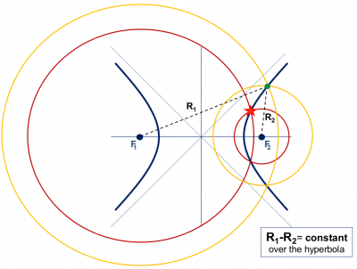Figure 2: An (unknown) offset [math]\displaystyle{ d \tau }[/math] in the ship's clock produces a shift in the measured ranges ([math]\displaystyle{ R_i\, = \,\rho_i\, +\, dr }[/math]) (or pseudoranges), varying the circumference radius. But, as both pseudoranges [math]\displaystyle{ R_1\, and\, R_2 }[/math] have been measured with the same clock, this offset cancels on the difference of ranges [math]\displaystyle{ R_1\, - \,R_2 = \rho_1\, - \,\rho_2\, = \,constant. }[/math] Thence, the ship is located at a branch of the hyperbola [math]\displaystyle{ R_1\, - \,R_2\, =\, constant. }[/math]

A third lighthouse will reduce the uncertainty in the ship position to only two possible solutions. Such solutions are given by the intersection of two hyperbolas as it is illustrated in figure 3. Notice that, after estimating the ship coordinates, its clock offset can be found from equation (1).

Figure 3: 2-D positioning with an unknown user clock offset.

To complete this analysis, the figure 1.4 shows another geometrical construction where the solution is in the centre of a circle, with radius equal to the clock offset [math]\displaystyle{ d r=v \cdot d \tau }[/math], and which is tangent to the three circles of radii [math]\displaystyle{ \rho_i }[/math] and centred in the lighthouses.

Figure 4: Geometrical view 2-D positioning, complementing the figure 3.

Finally, and in order to simplify the explanation, let's go back to the situation of figure 1 where the ship and lighthouses clocks are assumed fully synchronised. If the range measurements were perfect, the sailor could determine his position as the intersection point of the two circles centred at F1 and F2 lighthouses. However, the measurements are not exact, having some measurement error [math]\displaystyle{ \varepsilon }[/math]. Figures 5 and 6 illustrate how this measurement error is translated to the coordinates estimate as an uncertainty region, which depends on the geometry defined by the ship and lighthouses relative positions.

Figure 5: The measurement noise [math]\displaystyle{ \varepsilon }[/math] is translated to the position estimate as an uncertainty region.

Translation to the 3-D GNSS positioning

Although the preceding example corresponds to a two-dimensional case, the basic principle is the same in GNSS:

• Satellites (as the lighthouses): In the case of the lighthouses, one assumes that their coordinates are known. In the case of the GNSS satellites, the coordinates are calculated from the navigation data (ephemeris) transmitted by the satellites (see GNSS signal, Time References, Coordinate Systems and GNSS Satellites Orbit)

• Pseudorange measurements: In GNSS positioning, as well as in the example, distances between receiver and satellites are measured from the traveling time of a signal (in GNSS, an electromagnetic wave) from the satellite to the receiver (see GNSS signal, GNSS Basic Observables and Combination of GNSS Measurements)

Other comments:

• Clocks synchronisation: The satellite clocks are one of the most critical components of a GNSS system. In order to assure the stability of such clocks, GNSS satellites are equipped with atomic oscillators with high daily stabilities [math]\displaystyle{ \Delta f\, / \, f\, \simeq\, 10^{-13}\, -\, 10^{-14} }[/math]. However, despite this high stability satellite clocks accumulate some offsets along time. The satellite clock offsets are continuously estimated by the Ground Segment and transmitted to the users to correct the measurements (see GNSS Basic Observables and Combination of GNSS Measurements). The receivers, on the other hand, are equipped with quartz-based clocks, much more economical but with a poorer stability (about 10^-9). This inconvenience is overcome by estimating its clock offset together with the receiver coordinates, as in the previous example.
• From 2-D to 3-D positioning: It is not difficult to extend the previous 2-D geometrical construction to 3-D case of GNSS positioning, and to show that at least 4 satellites are needed to compute the three receiver coordinates plus clock. In this case, the previous circles and hyperbolas are generalised to spheres and hyperboloids, which intersect in two possible solutions. For a ground receiver, one of such solutions is on the earth's surface and the other far away in the space. An algebraic method to compute these two solutions (the Bancroft's method). Nevertheless, the usual way to solve this non linear problem is to linearise the equations around an approximate user position and solve iteratively (see Solving navigation equations).
• Dilution of precision (DOP): The geometry of the satellites, i.e., how the user sees them, affects the positioning error. This is illustrated in figure 1.6, where the size and shape of the region change depending on their relative position. This effect is called Dilution Of Precision (DOP) and it is studied in Predicted Accuracy: Dilution of Precision.

Figure 6: DOP effect in positioning: 2-D illustration of the variation of the uncertainty region with the geometry.