Code-Carrier Divergence Effect

Fundamentals
Title	Code-Carrier Divergence Effect
Author(s)	J. Sanz Subirana, J.M. Juan Zornoza and M. Hernández-Pajares, Technical University of Catalonia, Spain.
Level	Advanced
Year of Publication	2012

Introduction

The time variation of the ionosphere introduces a bias in the single frequency smoothed code (Carrier-smoothing), due to the code-carrier divergence. This effect is analysed as follows: The single frequency code ([math]\displaystyle{ R_1) }[/math] and carrier ([math]\displaystyle{ \Phi_1 }[/math]) measurements can be written in a simplified form as (see Combining pairs of signals and clock definition):

[math]\displaystyle{ \begin{array}{l} R_1=r +I_1+\varepsilon_1 \\ \Phi_1=r -I_1+B_1+\epsilon_1 \\ \end{array} \qquad \mbox{(1)} }[/math]

where [math]\displaystyle{ r }[/math] includes all non-dispersive terms such as geometric range, satellite and receiver clock offset and tropospheric delay. [math]\displaystyle{ I_1 }[/math] represents the frequency dependent terms as the ionosphere and instrumentals delays. [math]\displaystyle{ B_1 }[/math] is the carrier phase ambiguity term, which is constant along continuous carrier phase arcs. [math]\displaystyle{ \varepsilon_1 }[/math] and [math]\displaystyle{ \epsilon_1 }[/math] account for the code and carrier thermal noise and multipath. Since the ionospheric term has opposite sign in code and carrier measurements, it does not cancel in the [math]\displaystyle{ R-\Phi }[/math] combination, but on the contrary, its effect is twofold. That is :

[math]\displaystyle{ R_1-\Phi_1=2I_1+B_1+ \varepsilon_1 \qquad \mbox{(2)} }[/math]

The noisy (but unambiguous) code pseudorange measurements can be smoothed with the precise (but ambiguous) carrier phase measurements through the Hatch filter (see Carrier-smoothing):

[math]\displaystyle{ \begin{array}{ll} \widehat{R}(k)&= \frac{1}{n} R(k)+ \frac{n-1}{n} \left [ \widehat{R}(k-1)+ \left( \Phi(k) - \Phi(k-1) \right) \right ]=\\[0.3cm] &= \Phi(k) +\frac{n-1}{n} \left (\widehat{R}(k-1)-\Phi(k-1)\right )+ \frac{1}{n} \left( R(k)-\Phi(k) \right)=\\[0.3cm] & =\Phi(k) + \frac{n-1}{n} \lt R - \Phi\gt _{(k-1)} + \frac{1}{n} \left ( R(k) - \Phi(k) \right )=\\[0.3cm] &= \Phi(k) + \lt R - \Phi \gt _{(k)} \end{array} \qquad \mbox{(3)} }[/math]

Substituting (2) in the Hatch filter equation (3), results:

[math]\displaystyle{ \widehat{R}_1(k)=\Phi_1(k) + \lt R_1-\Phi_1 \gt _{(k)}=r(k) -I_1(k) +B_1+ \langle 2I_1-B_1 \rangle_{(k)} \qquad \mbox{(4)} }[/math]

Since the carrier ambiguity term [math]\displaystyle{ B_1 }[/math] is a constant bias and the average [math]\displaystyle{ \langle \cdot \rangle }[/math] is a linear operator, [math]\displaystyle{ B_1 }[/math] cancels in the previous equation (4), which can be re-written as (where the ionosphere is a time varying term):

[math]\displaystyle{ \widehat{R}_1(k)=\Phi_1(k) + \lt R_1 - \Phi_1 \gt _{(k)} = r(k) + I_1(k) + \underbrace{2 \left (\langle I_1 \rangle_{(k)} -I_1(k) \right )}_{{bias}_{I}} \qquad \mbox{(5)} }[/math]

That is, the time varying ionosphere produces a bias in the single frequency carrier-smoothed code (code-carrier divergence effect), in such a way that the first equation of (1) becomes for the smoothed code [math]\displaystyle{ \widehat{R}_1 }[/math] as:

[math]\displaystyle{ \widehat{R}_1= r+I_1+bias_I+\nu_1 \qquad \mbox{(6)} }[/math]

where [math]\displaystyle{ \nu_1 }[/math] is the noise term after the filter smoothing.

Divergence Free smoother

With two frequency measurements, the ionospheric term can be removed from a combination of the two frequencies carriers. Thus, neglecting the carrier noise and multipath [math]\displaystyle{ \epsilon_1 }[/math] and [math]\displaystyle{ \epsilon_2 }[/math] in front to the code [math]\displaystyle{ \varepsilon_1 }[/math]:

[math]\displaystyle{ R_1- \Phi_1-2 \tilde{\alpha}_1 (\Phi_1-\Phi_2)= B_{12}+\varepsilon_1 \qquad \mbox{(7)} }[/math]

where

[math]\displaystyle{ \tilde{\alpha}_1=\frac{1}{(f_1/f_2)^2-1} }[/math].

Using the previous combination (7) in (3), instead of (2), a smoothed code is obtained, free from the code-carrier ionosphere divergence effect, but having the same ionospheric delay as the original unsmoothed code [math]\displaystyle{ R_1 }[/math]:

[math]\displaystyle{ \widehat{R}_1= r+I_1+\nu_{12} \qquad \mbox{(8)} }[/math]

where [math]\displaystyle{ \nu_{12} }[/math] is the noise after the filter smoothing.

This smoothed code is called divergence-free carrier smoothed code

To illustrate the induced bias by the time varying ionosphere divergence on the single frequency smoothed code, the C1 carrier-smoothed code is computed using the expression (2), affected by the ionosphere divergence, and (7), divergence-free. The results are depicted in figure 1, left, where the accumulated bias is shown for three different smoothing filter time lengths ([math]\displaystyle{ 1 }[/math] hour, [math]\displaystyle{ 6 }[/math] minutes and [math]\displaystyle{ 1 }[/math] minute). As it can be seen, largest time constant leads to largest biases regarding to the unsmoothed code. In the given example, this bias reaches up to more than [math]\displaystyle{ 1 }[/math] meter with the [math]\displaystyle{ 1 }[/math] hour time smoothing, and up to [math]\displaystyle{ 50\, cm }[/math] with the [math]\displaystyle{ 6 }[/math] minutes smoothing. Note that these values depend on the ionospheric activity. The ionospheric refraction associated to these figures (from shifted [math]\displaystyle{ \Phi_1-\Phi_2 }[/math] carrier phases in meters of L1 delay) is shown at the bottom left plot as reference.

The sinusoidal-like oscillations are due to the code multipath. These oscillations are smoothed by increasing the time constant, but thence, a larger ionospheric bias can be introduced for the single frequency receivers smoothing.

Ionosphere Free smoother

The previous combination (7) uses two frequency carriers ([math]\displaystyle{ \Phi_1 }[/math] ,[math]\displaystyle{ \Phi_2 }[/math]), but only a single frequency code ([math]\displaystyle{ R_1 }[/math]). Using both code and carrier dual frequency measurements, it is possible to remove the frequency dependent effects

[math]\displaystyle{ \Phi_{_{LC}}=\frac{f_1^2\;\Phi_{_{L1}}-f_2^2\;\Phi_{_{L2}}}{f_1^2-f_2^2}~~~~~;~~~~~ R_{_{PC}}=\frac{f_1^2\;R_{_{P1}}-f_2^2\;R_{_{P2}}}{f_1^2-f_2^2} \qquad \mbox{(9)} }[/math]

using the code and carrier ionosphere-free combinations ([math]\displaystyle{ R_{_{C}} }[/math], [math]\displaystyle{ \Phi_{_{C}} }[/math]), see equation (11) in Combining pairs of signals and clock definition. Thence, the equations (1) become:

[math]\displaystyle{ \begin{array}{l} R_{_{C}}=r + \varepsilon_{_C}\\ \Phi_{_{C}}=r + B_{_C}+ \epsilon_{_C} \qquad \mbox{(10)} \end{array} }[/math]

And now, using the previous ionosphere-free combinations of code and carrier, the equation (2) is now:

[math]\displaystyle{ R_{_{C}}-\Phi_{_{C}}=B_{_C}+\varepsilon_{_C} \qquad \mbox{(11)} }[/math]

Applying this combination as input in the Hatch filter (3), a smoothed solution fully free of the (first order) ionosphere is computed:

[math]\displaystyle{ \widehat{R}_{_{C}} = r +\nu_{_{C}} \qquad \mbox{(12)} }[/math]

where [math]\displaystyle{ \nu_{_{C}} }[/math] is the noise after the filter smoothing. This smoothed code is called (ionosphere-free) carrier smoothed code The right side of figure (1) shows the ionosphere free carrier smoothed solution computed using the same smoothing time constants as with the C1-code.

Figure 1: Carrier-smoothed codes with different time filter lengths: [math]\displaystyle{ 1 }[/math] hour (first row), [math]\displaystyle{ 6 }[/math] minutes (second row), [math]\displaystyle{ 1 }[/math] minute (third row). Left hand plots C1-smoothing. Right hand iono-free smoothing. Black curves (left and right hand plots) show ionosphere-free smoothing, which is affected only by the multipath and receiver code noise. The red curves (right hand plots) accumulate the bias due to the divergence of the ionosphere. The larger noise in the right hand plots is due to the ionosphere free combination of codes. The ionospheric delay variation, computed from [math]\displaystyle{ \Phi_{1}-\Phi_{2} }[/math] (shifted) is shown in the last row in meters of L1 signal delay.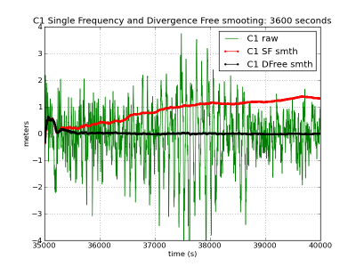

frameless	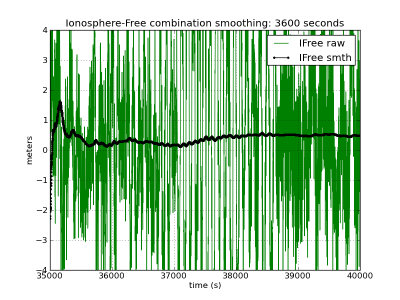frameless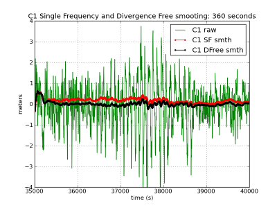
frameless	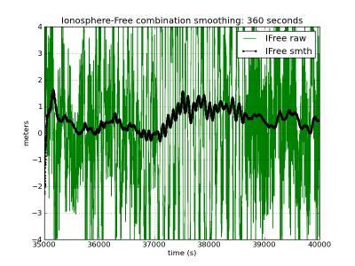frameless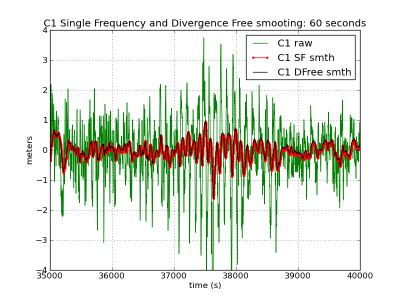
frameless	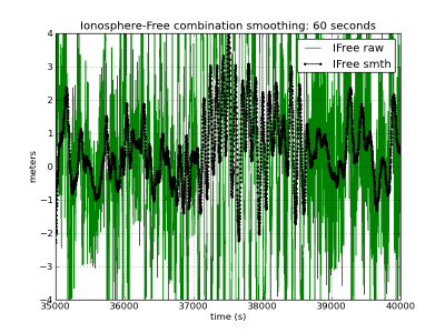frameless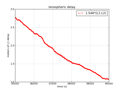
frameless	The left hand plots corresponds to the C1-carrier smoothing using equation (1), in red (affected by the code-carrier ionosphere divergence), and equation (2), in black (divergence-free). Right hand plots show the ionosphere-free smoothed code using the equation (7). The unsmoothed measurements in green correspond to [math]\displaystyle{ R_{1} }[/math] (left) and [math]\displaystyle{ R_{C} }[/math] (right) (zoom to [35000:40000] seconds).