If you wish to contribute or participate in the discussions about articles you are invited to contact the Editor
Solid Tides: Difference between revisions
Jaume.Sanz (talk | contribs) No edit summary |
Carlos.Lopez (talk | contribs) No edit summary |
||
| (4 intermediate revisions by one other user not shown) | |||
| Line 4: | Line 4: | ||
|Level=Advanced | |Level=Advanced | ||
|YearOfPublication=2011 | |YearOfPublication=2011 | ||
|Title={{PAGENAME}} | |Title={{PAGENAME}} | ||
}} | }} | ||
| Line 10: | Line 9: | ||
A simplified model for the tide displacement, but with few millimetres of accuracy, is given by the following expression (from IERS Conventions degree 2 tides displacement model --in-phase corrections--, see [Denis et al., 2004] <ref> [Denis et al., 2004] Denis, D., McCarthy and Petit, G., 2004. IERS Conventions (2003). IERS Technical Note 32 | A simplified model for the tide displacement, but with few millimetres of accuracy, is given by the following expression (from IERS Conventions degree 2 tides displacement model --in-phase corrections--, see [Denis et al., 2004] <ref> [Denis et al., 2004] Denis, D., McCarthy and Petit, G., 2004. IERS Conventions (2003). IERS Technical Note 32. IERS Convention Center, Frankfurt am Main.</ref>, page 79): | ||
:<math> | :<math> | ||
| Line 30: | Line 29: | ||
A small correction of latitude (<math>\varphi</math>) dependence can be considered in the <math>\displaystyle h_2</math> and <math>\displaystyle l_2</math> values of previous equation | A small correction of latitude (<math>\varphi</math>) dependence can be considered in the <math>\displaystyle h_2</math> and <math>\displaystyle l_2</math> values of previous equation (1) according to the expression: | ||
according to the expression: | |||
::<math> | ::<math> | ||
| Line 53: | Line 47: | ||
Finally, it must be taken into account that the previous equations provide the correction to obtain the coordinates relative to the "conventional tide free". To obtain the position relative to the "mean tide" the following vector must be added <ref group="footnotes"> According to the Resolution of 18th IAG General Assembly, 1983 (see [Denis et al., 2004] pages 9-10, and 83, the (degree 2 zonal) tidal potential contains a time independent (i.e., permanent) part, which is included in the geoid definition. Thence, the "mean tide" position is obtained after removing this part to the tidal displacement. This is done, by adding the vector (4) to the tidal displacement computed from equation (1).</ref>: | Finally, it must be taken into account that the previous equations provide the correction to obtain the coordinates relative to the "conventional tide free". To obtain the position relative to the "mean tide" the following vector must be added <ref group="footnotes"> According to the Resolution of 18th IAG General Assembly, 1983 (see [Denis et al., 2004] pages 9-10, and 83, the (degree 2 zonal) tidal potential contains a time independent (i.e., permanent) part, which is included in the geoid definition. Thence, the "mean tide" position is obtained after removing this part to the tidal displacement. This is done, by adding the vector in equation (4) to the tidal displacement computed from equation (1).</ref>: | ||
::<math> | ::<math> | ||
| Line 68: | Line 62: | ||
Notice that the radial component of this part can amount for about <math>-12</math> centimetres at the poles and about <math>+6</math> centimetres at the equator. | Notice that the radial component of this part can amount for about <math>-12</math> centimetres at the poles and about <math>+6</math> centimetres at the equator. | ||
An alternative set of equations describing a similar model implemented in GIPSY-OASIS II can be found in [Webb and Zumberge, 1993] <ref> [Webb and Zumberge, 1993] Webb, F. and Zumberge, J., 1993. An Introduction to GIPSY/OASIS-II. Jet Propulsion Laboratory, JPL, 4800 Oak Grove Drive, Pasadena, CA 91109.</ref> | An alternative set of equations describing a similar model implemented in GIPSY-OASIS II can be found in [Webb and Zumberge, 1993] <ref> [Webb and Zumberge, 1993] Webb, F. and Zumberge, J., 1993. An Introduction to GIPSY/OASIS-II. Jet Propulsion Laboratory, JPL, 4800 Oak Grove Drive, Pasadena, CA 91109.</ref>. | ||
Latest revision as of 11:41, 23 February 2012
| Fundamentals | |
|---|---|
| Title | Solid Tides |
| Author(s) | J. Sanz Subirana, J.M. Juan Zornoza and M. Hernández-Pajares, Technical University of Catalonia, Spain. |
| Level | Advanced |
| Year of Publication | 2011 |
Solid tides comprise the Earth's crust movement (and thus the receiver location coordinates variation) due to gravitational attracting forces produced by external bodies, mainly the sun and the moon. The Solid Tides produce vertical and horizontal displacements that can be expressed by spherical harmonics expansion ([math]\displaystyle{ \displaystyle m }[/math],[math]\displaystyle{ \displaystyle n }[/math]), characterised by the Love and Shida numbers [math]\displaystyle{ \displaystyle h_{mn} }[/math], [math]\displaystyle{ \displaystyle l_{mn} }[/math].
A simplified model for the tide displacement, but with few millimetres of accuracy, is given by the following expression (from IERS Conventions degree 2 tides displacement model --in-phase corrections--, see [Denis et al., 2004] [1], page 79):
- [math]\displaystyle{ \Delta {\mathbf r}= \sum_{j=2}^{3}{\frac{G\,M_j\,R_e^4}{G\,M_\oplus\,R_j^3}} \left \{h_2 \,\hat{\mathbf r} \left ( \frac{3}{2} (\hat{\mathbf R}_j \cdot \hat{\mathbf r})^2 -\frac{1}{2}\right) + 3\,l_2\,(\hat{\mathbf R}_j \cdot \hat{\mathbf r}) \left [\hat{\mathbf R}_j-(\hat{\mathbf R}_j \cdot \hat{\mathbf r})\,\hat{\mathbf r} \right ]\right \} \qquad\mbox{(1)} }[/math]
- [math]\displaystyle{ \Delta {\mathbf r} }[/math] is a site displacement vector in a Cartesian coordinates system.
- [math]\displaystyle{ G\,M_\oplus }[/math] is gravitational parameters of the earth.
- [math]\displaystyle{ G\,M_j }[/math] is gravitational parameters of the moon ([math]\displaystyle{ j = 2 }[/math]) and sun ([math]\displaystyle{ j = 3 }[/math]).
- ([math]\displaystyle{ M_{sun}/M_\oplus=332946.0 }[/math], [math]\displaystyle{ M_{moon}/M_\oplus=0.01230002 }[/math])
- [math]\displaystyle{ \hat{\mathbf R}_j }[/math], [math]\displaystyle{ \displaystyle R_j }[/math] are the unit vector from the geocentre to moon or sun and the magnitude of that vector.
- [math]\displaystyle{ \displaystyle R_e }[/math] is the earth's equatorial radius ([math]\displaystyle{ R_e=6378136.6\,m }[/math]).
- [math]\displaystyle{ \hat{\mathbf r} }[/math], [math]\displaystyle{ \displaystyle r }[/math] are the unit vector from the geocentre to the station and the magnitude of that vector.
- [math]\displaystyle{ \displaystyle h_2 }[/math] is the nominal degree 2 Love number ([math]\displaystyle{ \displaystyle h_2=0.6078 }[/math]).
- [math]\displaystyle{ \displaystyle l_2 }[/math] is the nominal degree 2 Shida number ([math]\displaystyle{ \displaystyle l_2=0.0847 }[/math]).
Notice that the radial (not vertical) component ([math]\displaystyle{ \displaystyle \hat{\mathbf r} }[/math]) is proportional to the Love number [math]\displaystyle{ \displaystyle h_2 }[/math], while the terms in [math]\displaystyle{ \displaystyle l_2 }[/math] corresponds to components orthogonal to the radial direction (not the horizontal plane).
A small correction of latitude ([math]\displaystyle{ \varphi }[/math]) dependence can be considered in the [math]\displaystyle{ \displaystyle h_2 }[/math] and [math]\displaystyle{ \displaystyle l_2 }[/math] values of previous equation (1) according to the expression:
- [math]\displaystyle{ \begin{array}{rl} h_2&= 0.6078-0.0006\left [(3 \sin^2\varphi-1)/2\right]\\[0.3cm] l_2&= 0.0847+0.0002\left [(3 \sin^2\varphi-1)/2\right] \end{array} \qquad\mbox{(2)} }[/math]
An additional refinement can be to take into account the additional contribution due to the degree 3 tides [Denis et al., 2004], page 80):
[math]\displaystyle{ \Delta {\mathbf r}= \sum_{j=2}^{3}{\frac{G\,M_j\,R_e^5}{G\,M_\oplus\,R_j^4}} \left \{h_3 \,\hat{\mathbf r} \left ( \frac{5}{2} (\hat{\mathbf R}_j \cdot \hat{\mathbf r})^3 -\frac{3}{2} (\hat{\mathbf R}_j \cdot \hat{\mathbf r})\right) + l_3\,\left (\frac{15}{2} (\hat{\mathbf R}_j \cdot \hat{\mathbf r})^2 - \frac{3}{2} \right ) \left [\hat{\mathbf R}_j-(\hat{\mathbf R}_j \cdot \hat{\mathbf r})\,\hat{\mathbf r} \right ]\right \} \qquad\mbox{(3)} }[/math]
where [math]\displaystyle{ \displaystyle h_3=0.292 }[/math] and [math]\displaystyle{ \displaystyle l_3=0.015 }[/math]. Only the moon's contribution ([math]\displaystyle{ j=2 }[/math]) need to be computed, because the contribution of sun ([math]\displaystyle{ j=3 }[/math]) is negligible. Nevertheless, also the moon's contribution to this degree 3 tide to the radial displacement does not exceed the [math]\displaystyle{ 1.7 }[/math] millimetres in radial and [math]\displaystyle{ 0.02 }[/math] millimetres in transversal components.
Finally, it must be taken into account that the previous equations provide the correction to obtain the coordinates relative to the "conventional tide free". To obtain the position relative to the "mean tide" the following vector must be added [footnotes 1]:
- [math]\displaystyle{ \begin{array}{ll} \left [-0.1206+0.0001\,P_2(\sin \varphi)\right ]P_2(\sin \varphi) \qquad\mbox{(m) radial direction}\\ \left [-0.0252+0.0001\,P_2(\sin \varphi)\right ]\sin 2\varphi \qquad\mbox{(m) north direction} \end{array} \qquad\mbox{(4)} }[/math]
where [math]\displaystyle{ P_2(\sin \varphi)=(3\,\sin^2\varphi-1)/2 }[/math].
Notice that the radial component of this part can amount for about [math]\displaystyle{ -12 }[/math] centimetres at the poles and about [math]\displaystyle{ +6 }[/math] centimetres at the equator.
An alternative set of equations describing a similar model implemented in GIPSY-OASIS II can be found in [Webb and Zumberge, 1993] [2].
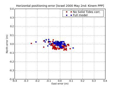
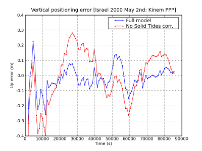
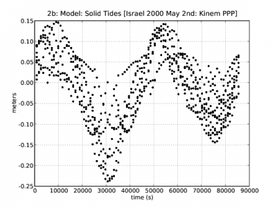
Figure 1 illustrates an example of the effect of the Solid Tides correction. The navigation solution computed using the solid tides correction is shown in blue and the solution without using this correction in red. The effect of solid tides displacement on range is shown in the second row at left.
Figure 1: Solid Tides: Range and position domain effect. First row shows the horizontal (left) and vertical (right) positioning error using (blue) or not using (red) the solid tides correction (from equations (1) to (3)). The effect on range of solid tides displacement is shown in the second row at left.
Notes
- ^ According to the Resolution of 18th IAG General Assembly, 1983 (see [Denis et al., 2004] pages 9-10, and 83, the (degree 2 zonal) tidal potential contains a time independent (i.e., permanent) part, which is included in the geoid definition. Thence, the "mean tide" position is obtained after removing this part to the tidal displacement. This is done, by adding the vector in equation (4) to the tidal displacement computed from equation (1).
References
- ^ [Denis et al., 2004] Denis, D., McCarthy and Petit, G., 2004. IERS Conventions (2003). IERS Technical Note 32. IERS Convention Center, Frankfurt am Main.
- ^ [Webb and Zumberge, 1993] Webb, F. and Zumberge, J., 1993. An Introduction to GIPSY/OASIS-II. Jet Propulsion Laboratory, JPL, 4800 Oak Grove Drive, Pasadena, CA 91109.


